
In partnership with


Join 400,000+ executives and professionals who trust The AI Report for daily, practical AI updates.
Built for business—not engineers—this newsletter delivers expert prompts, real-world use cases, and decision-ready insights.
No hype. No jargon. Just results.
🚀 Your Investing Journey Just Got Better: Premium Subscriptions Are Here! 🚀
It’s been 4 months since we launched our premium subscription plans at GuruFinance Insights, and the results have been phenomenal! Now, we’re making it even better for you to take your investing game to the next level. Whether you’re just starting out or you’re a seasoned trader, our updated plans are designed to give you the tools, insights, and support you need to succeed.
Here’s what you’ll get as a premium member:
Exclusive Trading Strategies: Unlock proven methods to maximize your returns.
In-Depth Research Analysis: Stay ahead with insights from the latest market trends.
Ad-Free Experience: Focus on what matters most—your investments.
Monthly AMA Sessions: Get your questions answered by top industry experts.
Coding Tutorials: Learn how to automate your trading strategies like a pro.
Masterclasses & One-on-One Consultations: Elevate your skills with personalized guidance.
Our three tailored plans—Starter Investor, Pro Trader, and Elite Investor—are designed to fit your unique needs and goals. Whether you’re looking for foundational tools or advanced strategies, we’ve got you covered.
Don’t wait any longer to transform your investment strategy. The last 4 months have shown just how powerful these tools can be—now it’s your turn to experience the difference.

Most traders draw Fibonacci levels by hand. That may be a problem.
Without a clear rule for where to start, it makes the implementation more difficult. This leads to subjective pivots and inconsistent angles.
This guide shows you how to automate the process using a volatility-based ZigZag approach meant for detecting significant swing highs and lows.
Once the key swing points are identified, Fibonacci fan lines are plotted to reflect the underlying geometry of the trend.
End-to-end Implementation Python Notebook provided below.
This article is structured as follows:
Why Fibonacci Fans Still Matter
Anchoring Fans with Price Structure
Python Implementation
What This Method Does Well and Where It Stops
1. Why Fibonacci Fans Still Matter
Fibonacci fans are rooted in number theory. The ratios they use — 0.382, 0.5, 0.618 — come from the Fibonacci sequence, a pattern studied since the 13th century.
These proportions appear in natural systems, architecture, and financial markets. Traders began applying them seriously in the 1970s, building on the popularity of Fibonacci retracements and extensions.
Fans take those same ratios but project them diagonally across time. You anchor one end to a major pivot and extend lines outward. Each line represents a structural zone where price may react
These levels often align with how trends expand and contract. That’s why they still matter: they reflect the natural ‘rhythm’ of price movement over time.
Take the Ethereum’s 2021 rally as an example. A fan anchored from the July low to the September high mapped key reaction zones during the pullback. Price stalled and bounced along the 38.2% and 61.8% lines.

Figure 1. Auto-generated Fibonacci fans for ETH-USD around the 2021 rally.
2. Anchoring Fans with Price Structure
The accuracy of any Fibonacci fan depends on where it’s anchored. If you get the pivot wrong, every line that follows loses meaning.
Our method uses recent volatility to filter out insignificant moves. Instead of hardcoding a minimum point difference or fixed time window, we define a relative threshold based on the asset’s price behavior.
We start by calculating a naive 10-bar range to estimate local volatility:

Then we convert this into a percentage deviation from the current close:
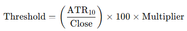
This threshold defines how large a move must be , relative to recent volatility , to qualify as a swing.
A higher multiplier captures only major pivots. A lower one makes the method more sensitive.
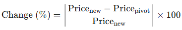
Each new bar is compared to the last confirmed pivot. If the percentage change exceeds the threshold, it’s marked as a new high or low.
If that value exceeds the threshold, the swing is valid. This logic gives us a clean list of swing points, filtered for significance.
Once pivots are detected, we sort them into highs and lows. From there, we define two anchor types:
Top fans: drawn from swing highs
Bottom fans: drawn from swing lows
3. Python Implementation
3.1. User Parameters
Define the ticker, date range, fan settings, and pivot selection logic.
You can choose whether to draw top fans (from swing highs), bottom fans (from swing lows), or both.
Each fan is anchored to a pivot you select, like the lowest low, second lowest, or third lowest point in the detected swings.
The same applies for highs. For example, setting top_origin = 2 anchors the fan from the second-highest high.
import numpy as np
import pandas as pd
import yfinance as yf
import matplotlib.pyplot as plt
import matplotlib.dates as mdates
plt.style.use("dark_background")

# PARAMETERS
TICKER = "ASML.AS"
START_DATE = "2023-06-01"
END_DATE = "2026-01-01"
INTERVAL = "1d"

# How sensitive the pivot detection should be.
# Higher values = fewer pivots (only big moves count), lower values = more pivots.
DEVIATION_MULT = 3.0

# Fibonacci fan levels to plot (as ratios)
FIB_LEVELS = [1.0, 0.75, 0.618, 0.5, 0.382, 0.25, 0.0]
REVERSE_FANS = False # If True, the fan lines will be flipped (mirrored logic).

# Control whether to show top fans (from highs) and/or bottom fans (from lows).
draw_top_fans = True
draw_bottom_fans = True

# Choose which pivot the fan lines should start from.
# Example: if you set this to 1, the fan will start from the highest (or lowest) pivot found.
# Set to 2 if you want the second highest/lowest, and so on.
# This lets you control which swing point to use for drawing the fans.
top_origin_selection = 1
bottom_origin_selection = 1


# FIB COLORS
fib_colors = {
    1.0: "#787b86",
    0.75: "#2196f3",
    0.618: "#009688",
    0.5: "#4caf50",
    0.382: "#81c784",
    0.25: "#f57c00",
    0.0: "#787b86"
}
3.2. Download Market Data
Pull historical price data from Yahoo Finance. Clean up column names, drop NaNs, and convert the index to datetime.
# DOWNLOAD DATA & SET DATETIME INDEX
df = yf.download(TICKER, start=START_DATE, end=END_DATE, interval=INTERVAL)
if df.empty:
    raise ValueError("No data returned from yfinance.")

if isinstance(df.columns, pd.MultiIndex):
    df.columns = [col[0] for col in df.columns]

df.dropna(subset=["Open","High","Low","Close"], inplace=True)
df.index = pd.to_datetime(df.index)
3.3. Volatility and Deviation Threshold
We calculate a simple 10-bar ATR to estimate recent price volatility. Instead of using the traditional ATR formula. We use the naive range outlined above:

This gives us the total price range over the last 10 bars. To make it relative to the current price, we convert it into a percentage-based deviation threshold:

This tells us how large a move needs to be, relative to current price and recent volatility to count as a meaningful swing.
The higher the DEVIATION_MULT, the fewer pivots will be detected.
# CALCULATE NAIVE ATR (10-bar) & DEVIATION THRESHOLD
df["ATR10"] = df["High"].rolling(10).max() - df["Low"].rolling(10).min()
df["dev_threshold"] = (df["ATR10"] / df["Close"]) * 100 * DEVIATION_MULT
3.4. Spot Swings with ZigZag Logic
Next, we scan through closing prices to detect significant swing highs and lows using percentage change from the last pivot.
If the price moves beyond the deviation threshold, we confirm a new pivot and store it as a tuple:
(index, price, isHigh)
index: bar positionprice: price at the pivotisHigh:Truefor a high,Falsefor a low
This ZigZag-style logic filters out minor fluctuations and captures only meaningful structural swings.
zigzag_indices = []  # stores tuples: (bar_index, price, isHigh)

last_pivot_idx = 0
last_pivot_price = df["Close"].iloc[0]

# Determine if first pivot is a high or low
last_pivot_is_high = df["Close"].iloc[1] < last_pivot_price

# Initialize with the first pivot
zigzag_indices.append((last_pivot_idx, last_pivot_price, last_pivot_is_high))

# Basic significance check based on % move vs threshold
def is_significant(dev_thr, old_price, new_price):
    return abs((new_price - old_price) / new_price)*100 > dev_thr

df_reset = df.reset_index(drop=True)

for i in range(1, len(df_reset)):
    cp = df_reset["Close"].iloc[i]
    dev_thr = df_reset["dev_threshold"].iloc[i]

    if last_pivot_is_high:
        if cp > last_pivot_price:
            # New local high; update current pivot
            last_pivot_idx = i
            last_pivot_price = cp
            zigzag_indices[-1] = (last_pivot_idx, last_pivot_price, last_pivot_is_high)
        else:
            if is_significant(dev_thr, last_pivot_price, cp):
                # Price dropped enough → confirm high, start new low
                zigzag_indices[-1] = (last_pivot_idx, last_pivot_price, True)
                last_pivot_idx = i
                last_pivot_price = cp
                last_pivot_is_high = False
                zigzag_indices.append((last_pivot_idx, last_pivot_price, last_pivot_is_high))
    else:
        if cp < last_pivot_price:
            # New local low; update current pivot
            last_pivot_idx = i
            last_pivot_price = cp
            zigzag_indices[-1] = (last_pivot_idx, last_pivot_price, last_pivot_is_high)
        else:
            if is_significant(dev_thr, last_pivot_price, cp):
                # Price rose enough → confirm low, start new high
                zigzag_indices[-1] = (last_pivot_idx, last_pivot_price, False)
                last_pivot_idx = i
                last_pivot_price = cp
                last_pivot_is_high = True
                zigzag_indices.append((last_pivot_idx, last_pivot_price, last_pivot_is_high))

# Ensure final pivot is updated
zigzag_indices[-1] = (last_pivot_idx, last_pivot_price, last_pivot_is_high)

# Abort if we didn’t find at least two pivots
if len(zigzag_indices) < 2:
    raise ValueError("Not enough pivots found.")
3.5. Anchor the Fans with Meaningful Pivots
Once pivots are detected, we split them into highs and lows:
Highs anchor top fans (resistance)
Lows anchor bottom fans (support)
For each fan, we do two things:
1. Select the origin: We sort the highs (descending) or lows (ascending) and pick the n-th pivot based on top_origin_selection or bottom_origin_selection.
2. Find the endpoint: We then locate the first opposite-type pivot that comes after the origin, e.g. a low after a high. This makes sure the fan represents a real price swing, not a random connection.
If no valid endpoint is found, we skip the fan to avoid drawing misleading lines.
# Split pivots into highs and lows
all_highs = [(i, p) for (i, p, h) in zigzag_indices if h]
all_lows = [(i, p) for (i, p, h) in zigzag_indices if not h]

# Sort: highest highs first, lowest lows first
all_highs_sorted = sorted(all_highs, key=lambda x: x[1], reverse=True)
all_lows_sorted = sorted(all_lows, key=lambda x: x[1])

# Pick the nth-highest pivot, or fallback to last one if n is too large
def pick_nth_high(sorted_highs, n):
    if not sorted_highs:
        return None, None
    return sorted_highs[n - 1] if n <= len(sorted_highs) else sorted_highs[-1]

# Pick the nth-lowest pivot, or fallback to last one if n is too large
def pick_nth_low(sorted_lows, n):
    if not sorted_lows:
        return None, None
    return sorted_lows[n - 1] if n <= len(sorted_lows) else sorted_lows[-1]

# Find the first opposite pivot (high vs low) after a given index
def find_next_opposite_pivot(origin_idx, origin_is_high):
    for (i, p, h) in zigzag_indices:
        if i > origin_idx and h != origin_is_high:
            return (i, p)
    return (None, None)

# Top fan: start from selected high pivot, end at next low after it
top_origin_idx, top_origin_price = pick_nth_high(all_highs_sorted, top_origin_selection)
top_end_idx, top_end_price = find_next_opposite_pivot(top_origin_idx, True)

# Bottom fan: start from selected low pivot, end at next high after it
bottom_origin_idx, bottom_origin_price = pick_nth_low(all_lows_sorted, bottom_origin_selection)
bottom_end_idx, bottom_end_price = find_next_opposite_pivot(bottom_origin_idx, False)

# Debug prints to confirm what’s being used
print("Top origin:", (top_origin_idx, top_origin_price))
print("Top end:", (top_end_idx, top_end_price))
print("Bottom origin:", (bottom_origin_idx, bottom_origin_price))
print("Bottom end:", (bottom_end_idx, bottom_end_price))
Top origin: (285, np.float64(995.8659057617188))
Top end: (468, np.float64(606.0))
Bottom origin: (83, np.float64(535.7083129882812))
Bottom end: (285, np.float64(995.8659057617188))
3.6. Project Fibonacci Geometry
Finally, we define a function to draw Fibonacci fan lines using the selected pivot pairs , an origin and an endpoint.
Each line starts from the origin and extends outward at an angle based on a specific Fibonacci level.
For a given Fibonacci level L, the projected price at the endpoint is:

This gives the vertical price target the fan line should reach. To plot it on a time-based chart, we calculate the slope:
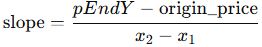
x1 is the origin date (as a number).
x2 is the endpoint date (as a number).
We then extend the line forward in time using this slope.
def extended_fib_fan_price(ax, origin_i, origin_p, end_i, end_p, fib_level, color, label):
    """
    Draws a single Fibonacci fan line from origin to projected future price based on fib_level.
    """

    # If any input is missing, skip drawing
    if None in (origin_i, end_i, origin_p, end_p):
        print(f"{label} => cannot draw line (missing pivot).")
        return

    origin_t = df.index[origin_i]
    end_t = df.index[end_i]

    x1 = mdates.date2num(origin_t)
    x2 = mdates.date2num(end_t)

    if x2 <= x1:
        # Protect against zero or negative time difference
        print(f"{label} => skipping because end <= origin in time.")
        return

    # Project a vertical price at the given Fibonacci level
    if not REVERSE_FANS:
        p_end_y = origin_p + (end_p - origin_p) * fib_level
    else:
        p_end_y = origin_p + (end_p - origin_p) * (1 - fib_level)

    # Compute slope based on time difference
    slope = (p_end_y - origin_p) / (x2 - x1)

    # Extend the line to the last date in the dataset
    final_time_num = mdates.date2num(df.index[-1])
    final_y = origin_p + slope * (final_time_num - x1)

    # Optional debug output
    print(f"{label}: origin=({origin_t}, {origin_p:.2f}), end=({end_t}, {end_p:.2f}),"
          f" pEndY={p_end_y:.2f}, slope={slope:.4f}")

    # Draw the line from origin to projected future point
    ax.plot([origin_t, mdates.num2date(final_time_num)],
            [origin_p, final_y],
            color=color, linewidth=1, label=label)
3.7. Visualize Price Structure
pPlot the price chart, all detected pivots, and draw the selected Fib fans.
fig, ax = plt.subplots(figsize=(16,8))
ax.plot(df.index, df["Close"], color="silver", lw=1.5, label="Close")

for (i, p, isHigh) in zigzag_indices:
    c = "orange" if isHigh else "cyan"
    ax.scatter(df.index[i], p, s=40, color=c, zorder=10)

if draw_top_fans and top_origin_idx is not None:
    for lvl in FIB_LEVELS:
        col = fib_colors.get(lvl, "white")
        extended_fib_fan_price(ax, top_origin_idx, top_origin_price,
                               top_end_idx, top_end_price,
                               lvl, col, f"Top Fib {lvl}")

if draw_bottom_fans and bottom_origin_idx is not None:
    for lvl in FIB_LEVELS:
        col = fib_colors.get(lvl, "white")
        extended_fib_fan_price(ax, bottom_origin_idx, bottom_origin_price,
                               bottom_end_idx, bottom_end_price,
                               lvl, col, f"Bottom Fib {lvl}")

ax.xaxis.set_major_formatter(mdates.DateFormatter('%Y-%m-%d'))
plt.gcf().autofmt_xdate()

ax.set_title(f"Auto Fib Fans: {TICKER}", color="white")
ax.set_xlabel("Date", color="white")
ax.set_ylabel("Price", color="white")
ax.legend(facecolor="gray", fontsize=8)
ax.grid(True, alpha=0.3)
plt.tight_layout()
plt.show()
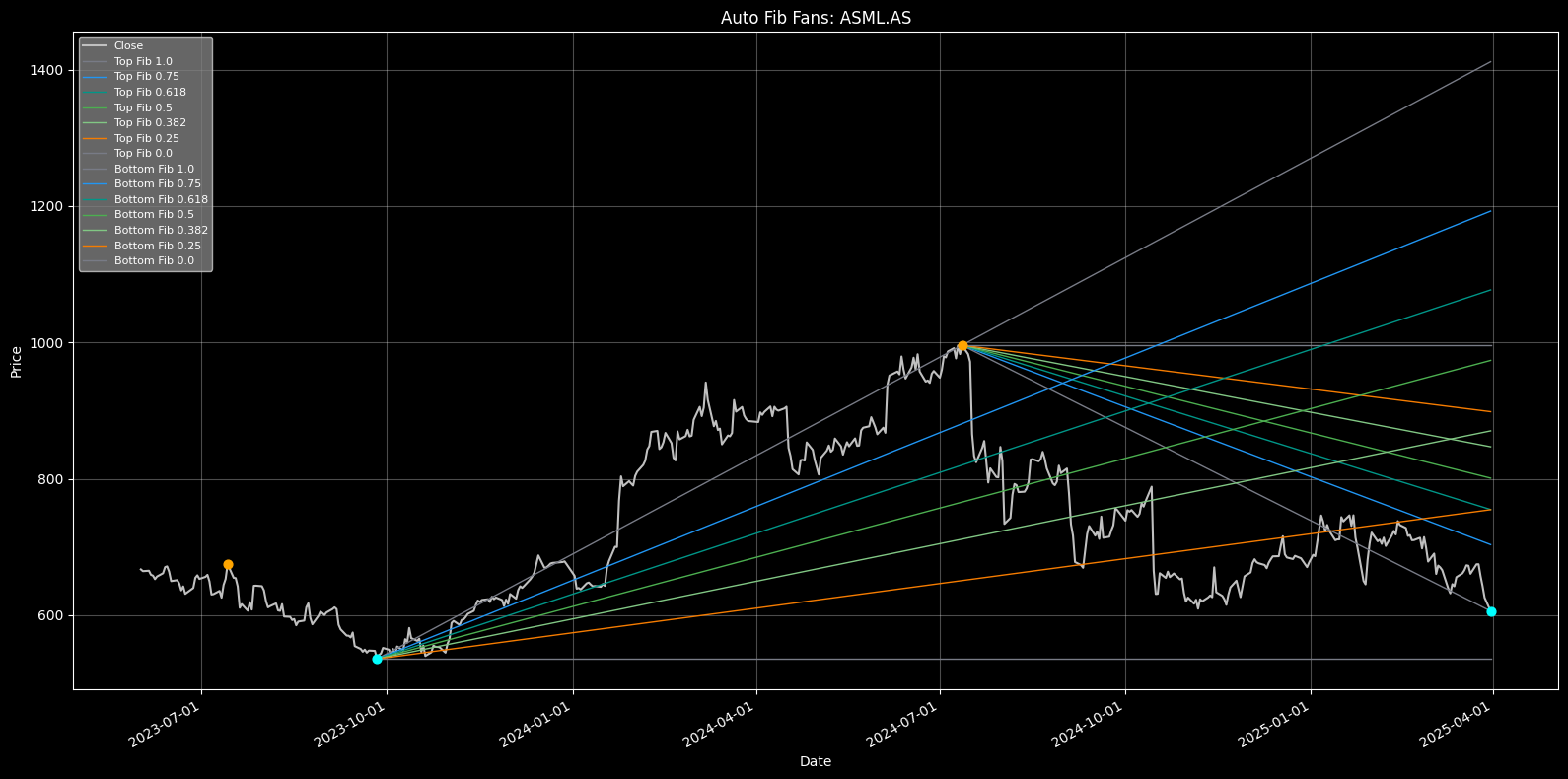
Figure 2. Auto-generated Fibonacci fans anchored to volatility-filtered pivot points. Top and bottom fans highlight potential structural zones based on recent price swings.
4. What This Method Does Well and Where It Stops
This method is great for anchoring fans to key price levels and adapts to the asset’s own behavior.
The pivot logic is transparent, rule-based, and repeatable. Every fan drawn has a clear structural justification.
It also gives you control. You can decide how sensitive the swing detection should be, how many fans to draw, and which pivot rank to use.
But it’s not a prediction tool. The fans don’t tell you where price is going. They show you where price might react, based on recent structure.
In sideways or erratic markets, fan lines may not align with meaningful levels.