Gold hitting record highs

The price of gold keeps heating up. If the record-breaking year of 2024 wasn't enough, gold hit a major historic 2025 milestone by crossing the $3,000/ounce threshold!

Here are 3 Key Reasons:

1. Looming economic & political uncertainty

2. Increasing central bank demand

3. Rising National Debt - over $36 Trillion

So, could gold surge even higher?

According to a recent statement from Jeffrey Gundlach, famed American business man and investor… “Gold continues its bull market that we’ve been talking about for a couple of years, ever since it was down to $1,800.” He expects gold to reach $4,000/oz.

Is it time you learn more about precious metals?

Get all the answers in your free 2025 Gold & Silver Kit. Plus, if you request your free kit today, you could qualify for up to 10% Instant Match in Bonus Silver*.

Learn more >>

_{*Offer valid on qualified orders of Goldco premium products only. Receive up to 10% in free silver based on purchase amount; cannot be combined with other offers. Additional terms apply—see your customer agreement or contact your representative for details.}

In today’s dynamic financial markets, sophisticated portfolio management requires more than traditional buy-and-hold strategies. This article introduces a Python implementation that combines hierarchical risk clustering with an adaptive long/short strategy, specifically designed for managing a portfolio of high-growth tech stocks, known as the “Magnificent Seven” (Apple, Microsoft, Google, Amazon, NVIDIA, Meta, and Tesla).

The Core Concepts

Before diving into the code, let’s understand the key concepts this implementation brings together:

1. Hierarchical Risk Clustering (HRC): This technique groups assets based on their correlation patterns, helping us diversify risk more effectively than traditional methods.

2. Risk-Adaptive Long/Short Strategy: Instead of always being long, our implementation switches between long positions in tech stocks and short positions in the S&P 500 (SPY) based on risk signals.

3. Multiple Risk Metrics: We combine drawdown limits, Value at Risk (VaR), and volatility measures to create a comprehensive risk management framework.

Let’s break down the implementation step by step.

Class Structure and Initialization

class HRCLongShortManager:
    def __init__(self, start_date, n_clusters=3, confidence_level=0.99,
                 window=252, max_drawdown=-15):

Our class initializes with several key parameters:

• start_date: Beginning of our historical data period

• n_clusters: Number of asset groups for risk clustering (default: 3)

• confidence_level: Confidence level for VaR calculations (default: 99%)

• window: Rolling window for volatility calculations (default: 252 trading days)

• max_drawdown: Maximum allowed drawdown (default: -15%)

Read The Daily Upside. Stay Ahead of the Markets. Invest Smarter.

Most financial news is full of noise. The Daily Upside delivers real insights—clear, concise, and free. No clickbait, no fear-mongering. Just expert analysis that helps you make smarter investing decisions.

Join 1M+ readers today.

Data Collection and Preparation

The download_data method handles data acquisition and initial processing:

def download_data(self):
    symbols = self.magnificent_seven + ['SPY']
    df_list = []
    for symbol in symbols:
        try:
            data = yf.download(symbol, self.start_date)
            df = data['Adj Close']
            df_list.append(df)
        except Exception as e:
            print(f"Error downloading {symbol}: {e}")
            continue

This method:

1. Downloads historical data for our tech stocks and SPY

2. Uses adjusted closing prices to account for corporate actions

3. Calculates returns and adds temporal information

4. Separates SPY returns for our long/short strategy

Hierarchical Risk Clustering

The clustering process is implemented in calculate_clusters:

def calculate_clusters(self):
    corr_matrix = self.returns[self.magnificent_seven].corr()
    dist_matrix = np.sqrt(2 * (1 - corr_matrix))
    linkage_matrix = linkage(squareform(dist_matrix), method='ward')

This method:

1. Calculates correlation matrix between assets

2. Converts correlations to distances (higher correlation = shorter distance)

3. Applies hierarchical clustering using Ward’s method

4. Groups similar assets together based on their risk characteristics

Portfolio Weight Calculation

The calculate_weights method implements our weighting strategy:

def calculate_weights(self):
    variances = self.returns[self.magnificent_seven].var()
    inv_variances = 1 / variances
    self.weights = pd.Series(0, index=self.magnificent_seven)

Key features:

1. Uses inverse variance weighting within clusters

2. Ensures equal risk contribution between clusters

3. Automatically adjusts weights based on asset volatility

Risk Metrics and Trading Signals

Our risk management system, implemented in calculate_portfolio_metrics, combines multiple risk measures:

def calculate_portfolio_metrics(self):
    # Portfolio value and drawdown
    self.portfolio_value = (1 + self.portfolio_returns).cumprod() * 100
    self.drawdown = ((self.portfolio_value - self.rolling_max) / self.rolling_max) * 100

    # Volatility and VaR calculations
    self.daily_volatility = self.portfolio_returns.rolling(window=self.window).std()
    z_score = norm.ppf(1 - self.confidence_level)
    self.daily_var = self.daily_volatility * z_score

The system monitors:

1. Portfolio drawdown against maximum limits

2. Daily and weekly Value at Risk violations

3. Volatility trends at different time scales

Long/Short Strategy Implementation

The strategy switches between positions based on risk signals:

def backtest_portfolio(self):
    backtest = pd.DataFrame(index=self.portfolio_returns.index)
    backtest['Long_Position'] = (~backtest['Risk_Signal']).astype(int)
    backtest['Short_Position'] = backtest['Risk_Signal'].astype(int) * -1

When risk signals are triggered:

1. Exits long positions in tech stocks

2. Takes short positions in SPY

3. Maintains these positions until risk metrics improve

Performance Visualization and Analysis

The code includes comprehensive visualization capabilities:

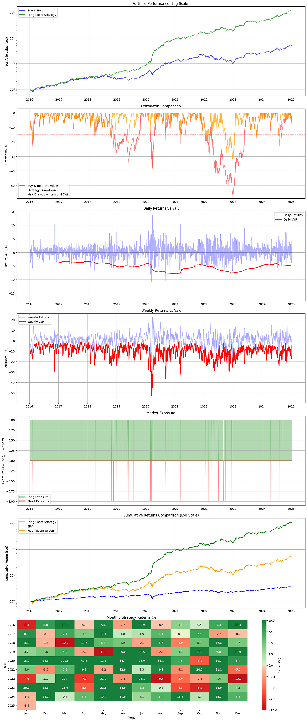
def plot_portfolio_analysis(self, backtest):
    fig, axes = plt.subplots(7, 1, figsize=(15, 35))
    # Performance plot
    axes[0].semilogy(backtest.index, backtest['Strategy_Equity'],
                     label='Long-Short Strategy', color='green', alpha=0.7)

Key visualizations include:

1. Portfolio performance on a log scale

2. Drawdown comparison with benchmark

3. VaR violations and risk metrics

4. Market exposure over time

5. Monthly returns heatmap with custom color scaling

Performance Statistics

The implementation calculates comprehensive performance metrics:

def _calculate_performance_stats(self, backtest, years, trading_days, initial_capital):
    stats = {
        'strategy': {
            'annual_return': ((1 + strategy_total_return/100) ** (1/years) - 1) * 100,
            'volatility': backtest['Strategy_Returns'].std() * np.sqrt(trading_days) * 100,
            'sharpe': stats['strategy']['annual_return'] / stats['strategy']['volatility'],
            'calmar': abs(stats['strategy']['annual_return'] / stats['strategy']['max_drawdown'])
        }
    }

These statistics include:

1. Total and annualized returns

2. Risk-adjusted metrics (Sharpe and Calmar ratios)

3. Exposure metrics and trading frequency

4. Comparison with buy-and-hold strategy

Practical Implementation

To use this portfolio manager:

if __name__ == "__main__":
    portfolio_manager = HRCLongShortManager('2016-01-01')
    returns = portfolio_manager.download_data()
    clusters = portfolio_manager.calculate_clusters()
    weights = portfolio_manager.calculate_weights()
    risk_signals = portfolio_manager.calculate_portfolio_metrics()
    backtest_results = portfolio_manager.backtest_portfolio()

Conclusion

This implementation offers a sophisticated approach to portfolio management by combining:

• Smart risk clustering for diversification

• Adaptive long/short positioning

• Comprehensive risk management

• Detailed performance analysis and visualization

The code is designed to be practical and suitable for both learning and real-world applications. While focused on the Magnificent Seven tech stocks, the approach can be adapted to other assets and markets.

The results are good enough, in theory. Also, did not used transactional costs.

=== Backtest Results (2016-2024) ===

Buy & Hold Statistics (Magnificent Seven):
Total Return: 4,748.37%
Annualized Return: 53.83%
Annualized Volatility: 36.57%
Sharpe Ratio: 1.47
Maximum Drawdown: -56.07%
Calmar Ratio: 0.96

Long-Short Strategy Statistics:
Total Return: 105,691.08%
Annualized Return: 116.57%
Annualized Volatility: 34.86%
Sharpe Ratio: 3.34
Maximum Drawdown: -31.50%
Calmar Ratio: 3.70
Long Exposure: 97.9%
Short Exposure: 2.1%
Number of Trades: 34