
In partnership with

Get Your Free ChatGPT Productivity Bundle

Mindstream brings you 5 essential resources to master ChatGPT at work. This free bundle includes decision flowcharts, prompt templates, and our 2025 guide to AI productivity.
Our team of AI experts has packaged the most actionable ChatGPT hacks that are actually working for top marketers and founders. Save hours each week with these proven workflows.
It's completely free when you subscribe to our daily AI newsletter.
🚀 Your Investing Journey Just Got Better: Premium Subscriptions Are Here! 🚀
It’s been 4 months since we launched our premium subscription plans at GuruFinance Insights, and the results have been phenomenal! Now, we’re making it even better for you to take your investing game to the next level. Whether you’re just starting out or you’re a seasoned trader, our updated plans are designed to give you the tools, insights, and support you need to succeed.
Here’s what you’ll get as a premium member:
Exclusive Trading Strategies: Unlock proven methods to maximize your returns.
In-Depth Research Analysis: Stay ahead with insights from the latest market trends.
Ad-Free Experience: Focus on what matters most—your investments.
Monthly AMA Sessions: Get your questions answered by top industry experts.
Coding Tutorials: Learn how to automate your trading strategies like a pro.
Masterclasses & One-on-One Consultations: Elevate your skills with personalized guidance.
Our three tailored plans—Starter Investor, Pro Trader, and Elite Investor—are designed to fit your unique needs and goals. Whether you’re looking for foundational tools or advanced strategies, we’ve got you covered.
Don’t wait any longer to transform your investment strategy. The last 4 months have shown just how powerful these tools can be—now it’s your turn to experience the difference.

Photo by CHUTTERSNAP on Unsplash
In investing, the task of portfolio optimization (PO) involves balancing the trade-off between risk and return, where portfolio return is maximized while financial risk (standard deviation) is minimized.
An optimally diversified portfolio can be constructed using the Monte Carlo simulation method in the spirit of the Markowitz original mean- variance optimizing framework, with one of the conditions being that asset weights in the portfolio sum to 1.
This PO can be intuitively and efficiently presented in Python by making use of the following sequence of 4 steps [1]:
Setting some key variables and fetching the stock data.
Calculating stock/benchmark daily returns and risks.
Generating a large number of randomly distributed portfolios to simulate the MPT efficient frontier [2] in the risk-return domain.
Comparing the optimal portfolio (best performer) and the market proxy values (benchmark) within the accepted risk zone.
Ideally, the resulting universe of assets and portfolios should lie on the efficient frontier [2].
In practice, using only historical data for covariance and correlation can lead to errors in PO because past performance is no guarantee of future results [3]. Besides, when you measure correlation and how you measure it has a large bearing on the optimization output.
These limitations of PO underline the importance of combining the Markowitz model with a comprehensive understanding of market dynamics and trends.
In this post, we’ll focus solely on the beginner-friendly specifics of the aforementioned workflow without investigating its drawbacks.
He’s already IPO’d once – this time’s different

Spencer Rascoff grew Zillow from seed to IPO. But everyday investors couldn’t join until then, missing early gains. So he did things differently with Pacaso. They’ve made $110M+ in gross profits disrupting a $1.3T market. And after reserving the Nasdaq ticker PCSO, you can join for $2.80/share until 5/29.
This is a paid advertisement for Pacaso’s Regulation A offering. Please read the offering circular at invest.pacaso.com. Reserving a ticker symbol is not a guarantee that the company will go public. Listing on the NASDAQ is subject to approvals. Under Regulation A+, a company has the ability to change its share price by up to 20%, without requalifying the offering with the SEC.
Step 1
Importing the necessary Python libraries, setting the key variables and fetching the selected stock data
import yfinance as yf
import pandas as pd
import numpy as np
import matplotlib.pyplot as plt

def download(tickers, start=None, end=None, actions=False, threads=True,
             group_by='column', auto_adjust=False, back_adjust=False,
             progress=True, period="max", show_errors=True, interval="1d", prepost=False,
             proxy=None, rounding=False, timeout=None, **kwargs):
    """Download yahoo tickers

   """

benchmark_ = ["^GSPC",]

portfolio_ = ['V', 'O', 'HD', 'MO', 'WM','NEE','PEP','CAT','UNH','MCD','XOM','UNP','CNQ','LMT','BLK','AAPL','MSFT','SBUX','ASML','COST']

start_date_ = "2022-01-01"
end_date_  = "2025-04-03"
number_of_scenarios = 10000

#Risk Boundary
delta_risk = 0.1


return_vector = []
risk_vector = []
distrib_vector = []

#Get Information from Benchmark and Portfolio
df = yf.download(benchmark_, start=start_date_, end=end_date_)
df2 = yf.download(portfolio_, start=start_date_, end=end_date_)

#Clean Rows with No Values on both Benchmark and Portfolio
df = df.dropna(axis=0)
df2 = df2.dropna(axis=0)

#Matching the Days
df = df[df.index.isin(df2.index)]
Steps 2–3
Generating random portfolios and calculating the average portfolio/benchmark return/risk
# Analysis of Benchmark
benchmark_vector = np.array(df[('Close', '^GSPC')])

#Create our Daily Returns
benchmark_vector = np.diff(benchmark_vector)/benchmark_vector[1:]

#Select or Final Return and Risk
benchmark_return = np.average(benchmark_vector)
benchmark_risk = np.std(benchmark_vector)

#Add our Benchmark info to our lists
return_vector.append(benchmark_return)
risk_vector.append(benchmark_risk)

# Analysis of Portfolio
portfolio_vector = np.array(df2['Close'])

#Create a loop for the number of scenarios we want:

for i in range(number_of_scenarios):
    #Create a random distribution that sums 1
    # and is split by the number of stocks in the portfolio
    random_distribution = np.random.dirichlet(np.ones(len(portfolio_)),size=1)
    distrib_vector.append(random_distribution)

    #Find the Closing Price for everyday of the portfolio
    portfolio_matmul = np.matmul(random_distribution,portfolio_vector.T)

    #Calculate the daily return
    portfolio_matmul = np.diff(portfolio_matmul)/portfolio_matmul[:,1:]

    #Select or Final Return and Risk
    portfolio_return = np.average(portfolio_matmul, axis=1)
    portfolio_risk = np.std(portfolio_matmul, axis=1)

    #Add our Benchmark info to our lists
    return_vector.append(portfolio_return[0])
    risk_vector.append(portfolio_risk[0])

#Create Risk Boundaries

min_risk = np.min(risk_vector)
max_risk = risk_vector[0]*(1+delta_risk)
risk_gap = [min_risk, max_risk]

#Portofolio Return and Risk Couple
portfolio_array = np.column_stack((return_vector,risk_vector))[1:,]
Step 4
Comparing the optimal portfolio (best performer) and the market proxy values (benchmark) within the accepted risk zone.
# Rule to create the best portfolio
# If the criteria of minimum risk is satisfied then:
if np.where(((portfolio_array[:,1]<= max_risk)))[0].shape[0]>1:
    min_risk_portfolio = np.where(((portfolio_array[:,1]<= max_risk)))[0]
    best_portfolio_loc = portfolio_array[min_risk_portfolio]
    max_loc = np.argmax(best_portfolio_loc[:,0])
    best_portfolio = best_portfolio_loc[max_loc]

# If the criteria of minimum risk is not satisfied then:
else:
    min_risk_portfolio = np.where(((portfolio_array[:,1]== np.min(risk_vector[1:]))))[0]
    best_portfolio_loc = portfolio_array[min_risk_portfolio]
    max_loc = np.argmax(best_portfolio_loc[:,0])
    best_portfolio = best_portfolio_loc[max_loc]
Creating final visualizations in the risk-return domain
#Visual Representation


trade_days_per_year = 252
risk_gap = np.array(risk_gap)*trade_days_per_year
best_portfolio[0] = np.array(best_portfolio[0])*trade_days_per_year
x = np.array(risk_vector)
y = np.array(return_vector)*trade_days_per_year

fig, ax = plt.subplots(figsize=(12, 8))

plt.rc('axes', titlesize=14)        # Controls Axes Title
plt.rc('axes', labelsize=14)        # Controls Axes Labels
plt.rc('xtick', labelsize=14)       # Controls x Tick Labels
plt.rc('ytick', labelsize=14)       # Controls y Tick Labels
plt.rc('legend', fontsize=14)       # Controls Legend Font
plt.rc('figure', titlesize=14)      # Controls Figure Title


ax.scatter(x, y, alpha=0.5,
           linewidths=0.1,
           edgecolors='black', s=20,
           label='Portfolio Scenarios'
            )

ax.scatter(x[0],
           y[0],
           color='red',
           linewidths=1,  s=180,
           edgecolors='black',
           label='Market Proxy Values')

ax.scatter(best_portfolio[1],
            best_portfolio[0],
            color='green',
            linewidths=1, s=180,
            edgecolors='black',
            label='Best Performer')

ax.axvspan(min_risk,
           max_risk,
           color='red',
           alpha=0.08,
           label='Accepted Risk Zone')

ax.set_ylabel("Yearly Portfolio Average Return (%)",fontsize=14)
ax.set_xlabel("Yearly Portfolio Standard Deviation",fontsize=14)

ax.axhline(y=0, color='black',alpha=0.5)

ax = plt.gca()
ax.legend(loc=0)
vals = ax.get_yticks()
ax.set_yticklabels(['{:,.2%}'.format(x) for x in vals])

PO in Action: Portfolio Scenarios, market Proxy Values, and Best Performer within the Accepted Risk Zone.
A mean-std plot was drawn for each portfolio, and the point corresponding to the highest Sharpe ratio can be identified on this plot.
Printing the output table of Stock % in Portfolio
#Output Table of Distributions
portfolio_loc = np.where((portfolio_array[:,0]==(best_portfolio[0]/trade_days_per_year))&(portfolio_array[:,1]==(best_portfolio[1])))[0][0]
best_distribution = distrib_vector[portfolio_loc][0].tolist()
d = {"Stock Name": portfolio_, "Stock % in Portfolio": best_distribution}
output = pd.DataFrame(d)
output = output.sort_values(by=["Stock % in Portfolio"],ascending=False)
output1=output.copy()
output= output.style.format({"Stock % in Portfolio": "{:.2%}"})
output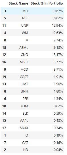
Stock % in Portfolio
Plotting the Treemap of the above portfolio
import squarify
import matplotlib.pyplot as plt
import seaborn as sb
episode_data =output1['Stock % in Portfolio']
anime_names = output1['Stock Name']
plt.figure(figsize=(12,12))
squarify.plot(episode_data, label=anime_names,color=sb.color_palette("Spectral",
                                     len(episode_data)),alpha=.7,pad=2)

plt.axis("off")
Optimal Portfolio Treemap.
Plotting the pie-chart of the above portfolio
output1.groupby(['Stock Name']).sum().plot(kind='pie', y='Stock % in Portfolio',legend=None,figsize=(16,14))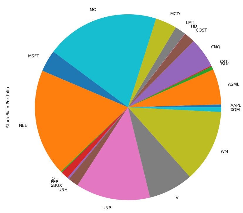
Pie-chart of the optimal portfolio
On top of the traditional asset classes of stocks and bonds, this analysis suggests that it is attractive for an investor to add Consumer Staples (MO), Clean Energy (NEE), Railroad Industry (UNP), and Environmental Services (WM).
By adding these asset classes, an investor almost captures the complete diversification benefit.
Conclusions
In the present post, we have discussed a basic PO approach and implemented an efficient algorithm for solving a class of (simplified) portfolio selection problems in Python.
The optimal model obtained in this study has an average return of 12.5% and a standard deviation of 0.011.
Its return is 4x higher than that of benchmark, and its standard deviation is the same as that of benchmark within the Accepted Risk Zone.
By optimizing the portfolio based on historical data, risks can be effectively diversified, resulting in relatively stable returns.
This study demonstrates that the Markowitz model has a certain degree of reliability and practical value in real-world applications.