
In partnership with


Join 400,000+ executives and professionals who trust The AI Report for daily, practical AI updates.
Built for business—not engineers—this newsletter delivers expert prompts, real-world use cases, and decision-ready insights.
No hype. No jargon. Just results.
🚀 Your Investing Journey Just Got Better: Premium Subscriptions Are Here! 🚀
It’s been 4 months since we launched our premium subscription plans at GuruFinance Insights, and the results have been phenomenal! Now, we’re making it even better for you to take your investing game to the next level. Whether you’re just starting out or you’re a seasoned trader, our updated plans are designed to give you the tools, insights, and support you need to succeed.
Here’s what you’ll get as a premium member:
Exclusive Trading Strategies: Unlock proven methods to maximize your returns.
In-Depth Research Analysis: Stay ahead with insights from the latest market trends.
Ad-Free Experience: Focus on what matters most—your investments.
Monthly AMA Sessions: Get your questions answered by top industry experts.
Coding Tutorials: Learn how to automate your trading strategies like a pro.
Masterclasses & One-on-One Consultations: Elevate your skills with personalized guidance.
Our three tailored plans—Starter Investor, Pro Trader, and Elite Investor—are designed to fit your unique needs and goals. Whether you’re looking for foundational tools or advanced strategies, we’ve got you covered.
Don’t wait any longer to transform your investment strategy. The last 4 months have shown just how powerful these tools can be—now it’s your turn to experience the difference.
It has recently been shown that the Python’s powerful framework of libraries and tools makes it ideal for implementing statistical arbitrage strategies (aka stat arb) [1].
Unlike traditional arbitrage, statistical arbitrage involves predicting and capitalizing on price movements over a time period. It focuses on immediate price gaps and exploits anticipated price adjustments over a longer period. This is where supervised Machine Learning (ML) comes into play [2]. Its essence lies in creating trained models that can automatically extract knowledge from market inefficiencies by taking advantage of pricing discrepancies between cointegrated assets.
The objective of this post is to improve ROI of statistical arbitrage strategies by invoking the SciKit-Learn ML classifiers [2].
In the sequel, we’ll consider the BBY and AAL close prices. According to the Macroaxis Correlation Matchups, these two securities move together with a correlation of +0.89.
Let’s get started!
He’s already IPO’d once – this time’s different

Spencer Rascoff grew Zillow from seed to IPO. But everyday investors couldn’t join until then, missing early gains. So he did things differently with Pacaso. They’ve made $110M+ in gross profits disrupting a $1.3T market. And after reserving the Nasdaq ticker PCSO, you can join for $2.80/share until 5/29.
This is a paid advertisement for Pacaso’s Regulation A offering. Please read the offering circular at invest.pacaso.com. Reserving a ticker symbol is not a guarantee that the company will go public. Listing on the NASDAQ is subject to approvals. Under Regulation A+, a company has the ability to change its share price by up to 20%, without requalifying the offering with the SEC.
Importing the necessary Python libraries and downloading the stock close prices 2020–2025
import yfinance as yf
import numpy as np
import pandas as pd
import statsmodels.api as sm
import matplotlib.pyplot as plt
from statsmodels.tsa.stattools import coint

from sklearn.model_selection import train_test_split
from sklearn.ensemble import RandomForestClassifier
from sklearn.neighbors import KNeighborsClassifier
from sklearn.naive_bayes import GaussianNB
from sklearn.metrics import accuracy_score

# Download stock data
tickers = ['AAL', 'BBY']
data = yf.download(tickers, start='2020-01-01')['Close']

# Preview the data
data.tail()

Ticker     AAL   BBY
Date
2025-05-19 11.86 71.599998
2025-05-20 11.65 71.150002
2025-05-21 11.24 70.150002
2025-05-22 11.40 70.760002
2025-05-23 11.19 69.919998
Plotting the stock close prices 2020–2025
plt.figure(figsize=(12, 6))
plt.plot(data['AAL'], label='AAL')
plt.plot(data['BBY'], label='BBY')
plt.title('Historical Stock Prices of AAL and BBY')
plt.xlabel('Date')
plt.ylabel('Price')
plt.legend()
plt.grid()
plt.show()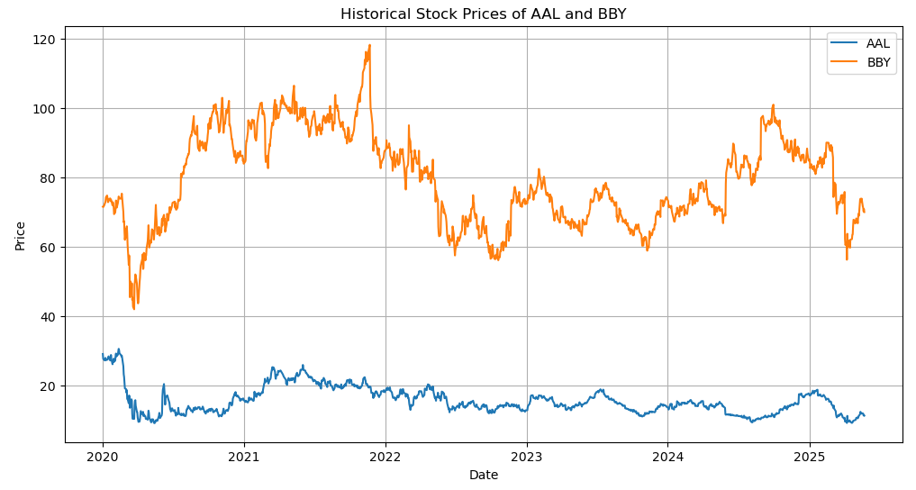
Historical Stock Prices of AAL and BBY
Performing the AAL-BBY cointegration test
score, p_value, _ = coint(data['AAL'], data['BBY'])

print(f'Cointegration test p-value: {p_value}')

# If p-value is low (<0.05), the pairs are cointegrated
if p_value < 0.05:
    print("The pairs are cointegrated.")
else:
    print("The pairs are not cointegrated.")

Cointegration test p-value: 0.009532269137951204
The pairs are cointegrated.
Calculating and plotting the spread between the two stocks
data['Spread'] = data['AAL'] - data['BBY']

# Plot the spread
plt.figure(figsize=(10, 6))
plt.plot(data.index, data['Spread'], label='Spread (AAL - BBY)')
plt.axhline(data['Spread'].mean(), color='red', linestyle='--', label='Mean')
plt.legend()
plt.xlabel('Date')
plt.ylabel('Spread')
plt.title('Spread between AAL and BBY')
plt.grid()
plt.show()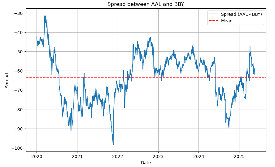
Spread between AAL and BBY
Defining the Z-score to normalize the spread and setting upper/lower thresholds for entering and exiting trades
# Define z-score to normalize the spread
data['Z-Score'] = (data['Spread'] - data['Spread'].mean()) / data['Spread'].std()

# Set thresholds for entering and exiting trades
upper_threshold = 2
lower_threshold = -2

# Initialize signals
data['Position'] = 0

# Generate signals for long and short positions
data['Position'] = np.where(data['Z-Score'] > upper_threshold, -1, data['Position'])  # Short the spread
data['Position'] = np.where(data['Z-Score'] < lower_threshold, 1, data['Position'])   # Long the spread
data['Position'] = np.where((data['Z-Score'] < 1) & (data['Z-Score'] > -1), 0, data['Position'])  # Exit

# Plot z-score and positions
plt.figure(figsize=(10, 6))
plt.plot(data.index, data['Z-Score'], label='Z-Score')
plt.axhline(upper_threshold, color='red', linestyle='--', label='Upper Threshold')
plt.axhline(lower_threshold, color='green', linestyle='--', label='Lower Threshold')
plt.legend()
plt.title('Z-Score of the Spread with Trade Signals')
plt.xlabel('Date')
plt.ylabel('Z-Score')
plt.grid()
plt.show()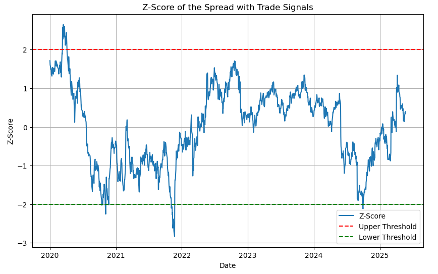
Z-Score of the Spread with Trade Signals
Calculating and plotting the strategy cumulative return (backtesting)
# Calculate daily returns
data['AAL_Return'] = data['AAL'].pct_change()
data['BBY_Return'] = data['BBY'].pct_change()

# Strategy returns: long spread means buying PEP and shorting KO
data['Strategy_Return'] = data['Position'].shift(1) * (data['AAL_Return'] - data['BBY_Return'])

# Cumulative returns
data['Cumulative_Return'] = (1 + data['Strategy_Return']).cumprod()

# Plot cumulative returns
plt.figure(figsize=(10, 6))
plt.plot(data.index, data['Cumulative_Return'], label='Cumulative Return from Strategy',lw=4)
plt.title('Cumulative Returns of Pairs Trading Strategy')
plt.legend()
plt.xlabel('Date')
plt.ylabel('Cumulative Return')
plt.grid()
plt.show()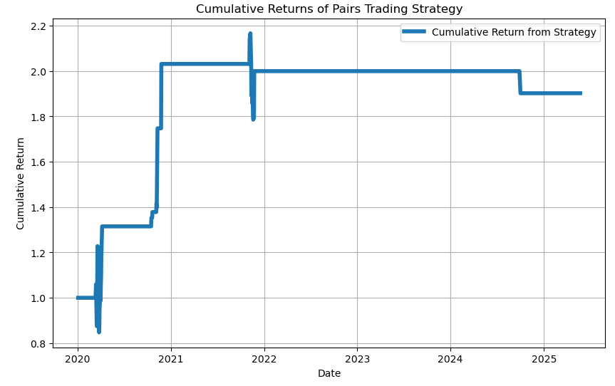
Cumulative Returns of Pairs Trading Strategy
Calculating the Sharpe ratio and max Drawdown of the strategy
# Calculate Sharpe Ratio
sharpe_ratio = data['Strategy_Return'].mean() / data['Strategy_Return'].std() * np.sqrt(252)
print(f'Sharpe Ratio: {sharpe_ratio}')

# Calculate max drawdown
cumulative_max = data['Cumulative_Return'].cummax()
drawdown = (cumulative_max - data['Cumulative_Return']) / cumulative_max
max_drawdown = drawdown.max()
print(f'Max Drawdown: {max_drawdown}')

Sharpe Ratio: 0.6280509157958919
Max Drawdown: 0.30985471721466773
Preparing our dataset for ML training
data['AAL_Return']=data['AAL_Return'].fillna(0)
data['BBY_Return']=data['BBY_Return'].fillna(0)
data['Cumulative_Return']=data['Cumulative_Return'].fillna(0)
data['Strategy_Return']=data['Cumulative_Return'].fillna(0)

data.head()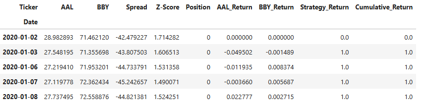
Input dataset for ML training
Defining the model features X (Returns) and the target variable y (Position)
X = data[['AAL_Return', 'BBY_Return']]
y = data['Position']
Splitting the data into the train/test sets with test_size=0.2
X_train, X_test, y_train, y_test = train_test_split(X, y, test_size=0.2, random_state=42)Implementing the Random Forest Classifier (RFC)
rf = RandomForestClassifier()
rf.fit(X_train, y_train)

# Make predictions
predictions = rf.predict(X_test)

# Calculate the accuracy of the model
accuracy = accuracy_score(y_test, predictions)
print(f'Accuracy of the Random Forest Classifier: {accuracy}')

Accuracy of the Random Forest Classifier: 0.9522058823529411
Using the test set to compare the cumulative strategy returns with/without RFC test predictions
s = pd.Series(predictions, index=y_test.index)

data['Test_Return'] = y_test.shift(1) * (data['AAL_Return'] - data['BBY_Return'])
data['RFC_Return'] =s.shift(1) * (data['AAL_Return'] - data['BBY_Return'])
# Cumulative returns
data['Test_Cumulative_Return'] = (1 + data['Test_Return']).cumprod()
data['RFC_Cumulative_Return'] = (1 + data['RFC_Return']).cumprod()
# Plot cumulative returns
plt.figure(figsize=(10, 6))
plt.plot(data.index, data['Test_Cumulative_Return'], label='Test Cumulative Return',lw=4)
plt.plot(data.index, data['RFC_Cumulative_Return'], label='RFC Cumulative Return',lw=4)
plt.title('Test Data: Cumulative Returns of Pairs Trading Strategy with/without ML Classifier')
plt.legend()
plt.xlabel('Date')
plt.ylabel('Cumulative Return')
plt.grid()
plt.show()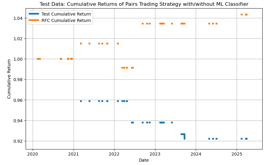
Test set: cumulative strategy returns with/without RFC predictions
Observe a 8% loss and 4% profit in the test data strategy without/with RFC, respectively.
Implementing the KNN Classifier
rf = KNeighborsClassifier(n_neighbors=3)

rf.fit(X_train, y_train)

# Make predictions
predictions = rf.predict(X_test)

# Calculate the accuracy of the model
accuracy = accuracy_score(y_test, predictions)
print(f'Accuracy of KNN: {accuracy}')

Accuracy of KNN: 0.9632352941176471
Using the test set to compare the cumulative strategy returns with/without KNN test predictions
s = pd.Series(predictions, index=y_test.index)

# Strategy returns
data['Test_Return'] = y_test.shift(1) * (data['AAL_Return'] - data['BBY_Return'])
data['KNN_Return'] =s.shift(1) * (data['AAL_Return'] - data['BBY_Return'])
# Cumulative returns
data['Test_Cumulative_Return'] = (1 + data['Test_Return']).cumprod()
data['KNN_Cumulative_Return'] = (1 + data['KNN_Return']).cumprod()
# Plot cumulative returns
plt.figure(figsize=(10, 6))
plt.plot(data.index, data['Test_Cumulative_Return'], label='Test Cumulative Return',lw=4)
plt.plot(data.index, data['KNN_Cumulative_Return'], label='KNN Cumulative Return',lw=4)
plt.title('Test Data: Cumulative Returns of Pairs Trading Strategy with/without ML Classifier')
plt.legend()
plt.xlabel('Date')
plt.ylabel('Cumulative Return')
plt.grid()
plt.show()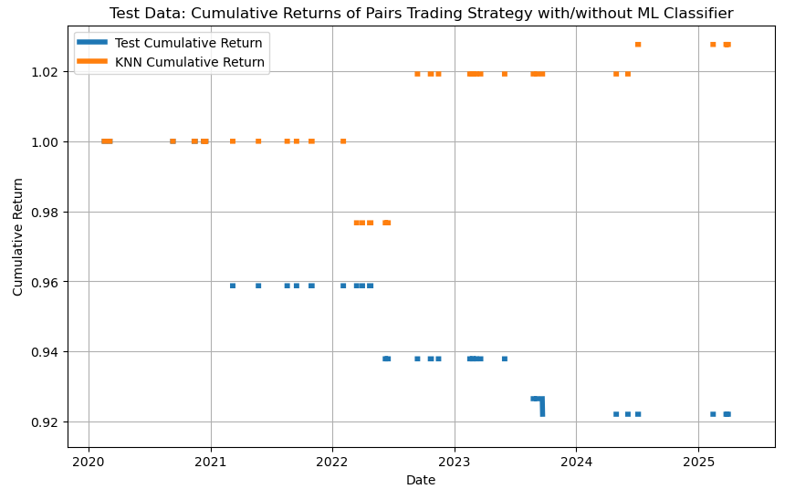
Test set: cumulative strategy returns with/without KNN predictions
Observe a 8% loss and ~3% profit in the test data strategy without/with KNN, respectively.
Calculating the Sharpe ratio and max Drawdown for the test set without ML and with RFC/KNN predictions
#Test set without ML

# Calculate Sharpe Ratio
sharpe_ratio = data['Test_Return'].mean() / data['Test_Return'].std() * np.sqrt(252)
print(f'Sharpe Ratio: {sharpe_ratio}')

# Calculate max drawdown
cumulative_max = data['Test_Cumulative_Return'].cummax()
drawdown = (cumulative_max - data['Test_Cumulative_Return']) / cumulative_max
max_drawdown = drawdown.max()
print(f'Max Drawdown: {max_drawdown}')

Sharpe Ratio: -0.7233058926453204
Max Drawdown: 0.0817497058494896


#Test set with RFC


# Calculate Sharpe Ratio
sharpe_ratio = data['RFC_Return'].mean() / data['RFC_Return'].std() * np.sqrt(252)
print(f'Sharpe Ratio: {sharpe_ratio}')

# Calculate max drawdown
cumulative_max = data['RFC_Cumulative_Return'].cummax()
drawdown = (cumulative_max - data['RFC_Cumulative_Return']) / cumulative_max
max_drawdown = drawdown.max()
print(f'Max Drawdown: {max_drawdown}')

Sharpe Ratio: 0.7330645837264052
Max Drawdown: 0.023280253670126764

#Test set with KNN


# Calculate Sharpe Ratio
sharpe_ratio = data['KNN_Return'].mean() / data['KNN_Return'].std() * np.sqrt(252)
print(f'Sharpe Ratio: {sharpe_ratio}')

# Calculate max drawdown
cumulative_max = data['KNN_Cumulative_Return'].cummax()
drawdown = (cumulative_max - data['KNN_Cumulative_Return']) / cumulative_max
max_drawdown = drawdown.max()
print(f'Max Drawdown: {max_drawdown}')

Sharpe Ratio: 0.5483810027312457
Max Drawdown: 0.02328025367012676
Conclusions
In this post we employed supervised ML techniques [2] to improve ROI of the stat arb strategy applied to the cointegrated pair AAL-BBY 2020–2025.
We have used backtesting with Sharpe ratio and max Drawdown to evaluate the viability of our strategies on test data.
Our ML test results have confirmed that RFC can significantly improve ROI of stat arb (cf. 8% loss vs 4% profit without/with RFC test predictions, respectively) with 4 times lower max Drawdown.
It appears that RFC has slightly outperformed KNN in terms of ROI (cf. 4% and 3% profits, respectively).
It is interesting to see that both RFC and KNN yield the same 2% max Drawdown.
Robustness checks and sensitivity analyses will further corroborate these findings.