
In partnership with

StartEngine’s $30M Surge — Own a Piece Before June 26

Private markets are having a moment, thanks to companies like StartEngine.
The leading alternative investing platform is helping everyday investors like you access deals once reserved for VCs and insiders, including exposure to private market titans like OpenAI, Databricks, and Perplexity.¹
How’s it going? In Q1 2025, StartEngine pulled off $30M in revenue, its biggest quarter ever (based on unaudited financials).²
But StartEngine isn’t just a middleman. The company earns 20% carried interest on select pre-IPO offerings, unlocking value for shareholders when these deals succeed.³
How can you tap into this diversification play? By investing in StartEngine.
StartEngine has crowdfunded $85M+ to date, and you can join 45K+ shareholders before the company’s current round closes on June 26.
Reg A+ via StartEngine Crowdfunding, Inc. No BD/intermediary involved. Investment is speculative, illiquid & high risk. See OC and Risks on page.
🚀 Your Investing Journey Just Got Better: Premium Subscriptions Are Here! 🚀
It’s been 4 months since we launched our premium subscription plans at GuruFinance Insights, and the results have been phenomenal! Now, we’re making it even better for you to take your investing game to the next level. Whether you’re just starting out or you’re a seasoned trader, our updated plans are designed to give you the tools, insights, and support you need to succeed.
Here’s what you’ll get as a premium member:
Exclusive Trading Strategies: Unlock proven methods to maximize your returns.
In-Depth Research Analysis: Stay ahead with insights from the latest market trends.
Ad-Free Experience: Focus on what matters most—your investments.
Monthly AMA Sessions: Get your questions answered by top industry experts.
Coding Tutorials: Learn how to automate your trading strategies like a pro.
Masterclasses & One-on-One Consultations: Elevate your skills with personalized guidance.
Our three tailored plans—Starter Investor, Pro Trader, and Elite Investor—are designed to fit your unique needs and goals. Whether you’re looking for foundational tools or advanced strategies, we’ve got you covered.
Don’t wait any longer to transform your investment strategy. The last 4 months have shown just how powerful these tools can be—now it’s your turn to experience the difference.

Markets rarely repeat exactly, but they revisit historical patterns. This article shows how to turn those setups into today’s trading signals.
Here, we how to predict short-term price direction by comparing today’s market state to similar conditions in the past using unsupervised learning.
We use a custom K-nearest neighbors method with Lorentzian distance to track how technical patterns played out historically .
Instead of training a predictive model, we use ‘market memory’. We define each n number of bars bar by a set of 5 technical indicators.
Whe then compare recent patterns to hundreds of past ones. This is a more transparent signal-generation method. No training. No black-box models.
What Top Execs Read Before the Market Opens
The Daily Upside was built by investment pros to give execs the intel they need—no fluff, just sharp insights on trends, deals, and strategy. Join 1M+ professionals and subscribe for free.
End-to-end Implementation Python Notebook provided below.

This Article is structured as follows:
Trading on Pattern Memory Model
Getting the Data for Pattern Recall
Feature Engineering with Indicator Functions
Lorentzian Distance: A Smarter Similarity Measure
Training Labels and KNN Prediction
2. Trading on Pattern Memory
Instead of forecasting, we look backward and search for days in the past that resemble the market conditions we’re seeing now.
We then track what followed in those past cases. If similar setups often led to the same price moves, that suggests the possible direction of today.
This idea is based on non-parametric classification. No training, no optimization, no fitted model. Just memory-based reasoning.
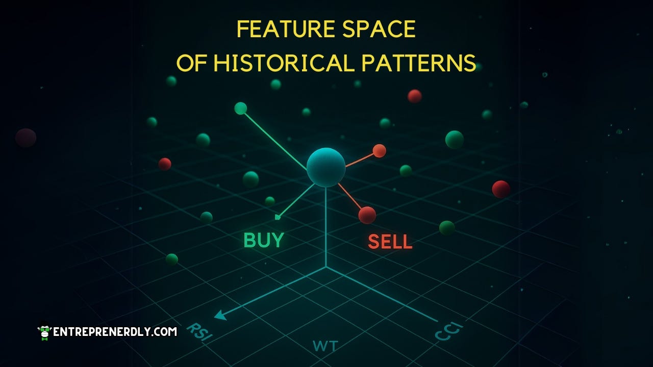
2.1 Market States as Feature Vectors
To compare market behavior over time, we need a way to encode each trading day numerically.
We do this by calculating 5 technical indicators from price data:
Relative Strength Index
Wave Trend
Commodity Channel Index
ADX (trend strength)
A second RSI with a shorter lookback
Each day becomes a vector in multi-dimensional space:

But instead of looking at just one day, we go further. We use a sliding window of 5 (adjustable) consecutive bars to capture short-term behavior.
That gives each observation more context. So the full feature vector becomes:

Each one is a flattened array of 25 numbers, i.e. 5 indicators over 5 bars. This becomes our representation of a “market state”.
2.2 Measuring Similarity with Lorentzian Distance
To compare today’s pattern with previous ones, we need a distance function.
Instead of using Euclidean distance, which can be thrown off by large deviations, we use Lorentzian distance, defined as:
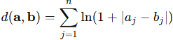
This function grows slowly as differences increase to be more tolerant of outliers and noise.
In simple terms, Lorentzian measures how similar the shape and magnitude of two market states are, without overreacting to a single volatile spike.
2.3 Find Similar Setups, Watch What Followed
Once we’ve encoded every market state and defined how to measure similarity, the process is simple:
For today’s vector, compare it to all previous ones within a lookback window, e.g. the last 200 bars.
Sort by Lorentzian distance to find the k-nearest past setups, e.g. the closest 100.
Assign labels based on what happened after those historical bars:
+1 if price rose within the next n bars, e.g. 4 bars
–1 if it fell
0 if it was flat
Then, just sum the labels:
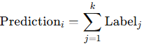
If the sum is positive, most similar past setups led to gains. If it’s negative, they led to losses. This output, therefore, becomes a directional signal.
3. Python Implementation
3.1. Get Data for Pattern Recall
We download daily price data for a given ticker. The data is cleaned and reset so that each row represents one trading bar.
import numpy as np
import pandas as pd
import yfinance as yf
import matplotlib.pyplot as plt
import matplotlib.dates as mdates

# DOWNLOAD DATA
TICKER     = "ASML.AS"
START_DATE = "2022-01-01"
END_DATE   = "2025-07-01"

df = yf.download(TICKER, start=START_DATE, end=END_DATE, interval="1d")
if df.empty:
    raise ValueError("No data returned from yfinance.")

# Flatten columns if multi-index
if isinstance(df.columns, pd.MultiIndex):
    df.columns = df.columns.get_level_values(0)

# Standard renaming/cleanup
df.rename(columns={"Open":"Open","High":"High","Low":"Low","Close":"Close","Volume":"Volume"}, inplace=True)
df.dropna(subset=["Close","High","Low"], inplace=True)
df["Date"] = df.index
df.reset_index(drop=True, inplace=True)
n = len(df)
3.2. Feature Engineering with Indicator Functions
We compute the 5 technical indicators from the price series. These serve as the features for comparing one market state to another.
Each indicator captures a different dimension of market structure, i.e. momentum, volatility, trend strength, and deviation.
Here’s how they’re defined in the code:
3.2.1 Relative Strength Index
RSI measures momentum by comparing the magnitude of recent gains to recent losses. It’s defined as:
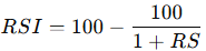
RS is the ratio of average gains to average losses over the last 14 bars.
3.2.2. Wave Trend Oscillator
Wave Trend is a smoothed oscillator based on the average price of each bar. It filters out noise using exponential moving averages:
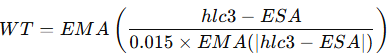
Here
and ESA is the EMA of hlc3.
3.2.3. Commodity Channel Index
CCI measures how far price deviates from its moving average:
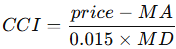
MA is the 20-bar moving average, and MD is the mean deviation from that average.
3.2.4. Average Directional Index
ADX quantifies trend strength. It’s based on directional movement indicators:

These are combined into the directional index:
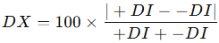
ADX is the EMA of DX over 14 bars. The higher it is, the stronger the trend.
3.2.5. Short-Term RSI
We also include a second RSI, calculated over just 9 bars, to capture faster momentum shifts.
# HELPER INDICATOR FUNCTIONS
def rsi(series, length=14):
    delta = series.diff()
    gain = delta.clip(lower=0)
    loss = -delta.clip(upper=0)
    avg_gain = gain.ewm(alpha=1/length, adjust=False).mean()
    avg_loss = loss.ewm(alpha=1/length, adjust=False).mean()
    rs = avg_gain / avg_loss
    return 100 - (100 / (1 + rs))

def wave_trend(hlc3, n1=10, n2=11):
    esa = hlc3.ewm(span=n1, adjust=False).mean()
    d = abs(hlc3 - esa).ewm(span=n1, adjust=False).mean()
    ci = (hlc3 - esa) / (0.015 * d)
    wt = ci.ewm(span=n2, adjust=False).mean()
    return wt

def cci(series, length=20):
    ma = series.rolling(length).mean()
    md = (series - ma).abs().rolling(length).mean()
    return (series - ma) / (0.015 * md)

def adx(df, length=14):
    high = df["High"]
    low = df["Low"]
    close = df["Close"]
    plus_dm = (high - high.shift(1)).clip(lower=0)
    minus_dm = (low.shift(1) - low).clip(lower=0)
    plus_dm[plus_dm < minus_dm] = 0
    minus_dm[minus_dm <= plus_dm] = 0

    tr1 = df["High"] - df["Low"]
    tr2 = abs(df["High"] - close.shift(1))
    tr3 = abs(df["Low"] - close.shift(1))
    tr = pd.concat([tr1, tr2, tr3], axis=1).max(axis=1)

    atr = tr.ewm(alpha=1/length, adjust=False).mean()
    plus_di = 100 * (plus_dm.ewm(alpha=1/length, adjust=False).mean() / atr)
    minus_di = 100 * (minus_dm.ewm(alpha=1/length, adjust=False).mean() / atr)
    dx = 100 * abs(plus_di - minus_di) / (plus_di + minus_di)
    return dx.ewm(alpha=1/length, adjust=False).mean()
3.3. Building the Feature Matrix
Calculate each indicator and store them as feature vectors for every bar. We’ll use these to compare current conditions against recent history.
Instead of using one bar at a time, we build feature vectors using a rolling window of n bars.
Each vector is a flattened set of indicator values from the current bar and the n-1 before it.
This captures short-term behavior and lets us compare multi-bar patterns instead of isolated bars.
# BUILD FEATURES
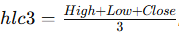
df["hlc3"] = (df["High"] + df["Low"] + df["Close"]) / 3.0
df["feat1"] = rsi(df["Close"], 14)
df["feat2"] = wave_trend(df["hlc3"], 10, 11)
df["feat3"] = cci(df["Close"], 20)
df["feat4"] = adx(df, 14)
df["feat5"] = rsi(df["Close"], 9)
# Build the original features matrix (each bar's indicators)
features = df[["feat1", "feat2", "feat3", "feat4", "feat5"]].to_numpy()
# We're using the last 5 bars instead of just 1
# For each point in time, we take the features from the current bar and the 4 before it
# Then we flatten that into one long vector.
# This way, we're comparing recent behavior — not just a single moment
window_length = 5
# Each new observation concatenates features from 5 consecutive bars.
features_windowed = np.array([
features[i - window_length + 1 : i + 1].flatten()
for i in range(window_length - 1, n)
])
n_window = features_windowed.shape[0]3.4. Lorentzian Distance: A Smarter Similarity Measure
To compare feature vectors, we use Lorentzian distance:
This measure gives the similarity between current bar and past bars (‘feature states’).
# LORENTZIAN DISTANCE
def lorentzian_distance(a, b):
    return np.sum(np.log1p(np.abs(a - b)))
3.5. Generate Training Labels via Historical Outcomes
For each past market state, we assign a label based on what the price did in the near future. Specifically, over the next 4 bars:
This gives us a simple way to score the outcome of each historical setup. So later, when we find similar patterns, we already know how they turned out.
# TRAINING LABELS
# barLookahead = 4 => we compare close[i+4] with close[i]
# If up => label=+1, if down => label=-1, else 0
barLookahead = 4
y_train = np.zeros(n, dtype=int)
for i in range(n - barLookahead):
    if df["Close"].iloc[i + barLookahead] > df["Close"].iloc[i]:
        y_train[i] = 1
    elif df["Close"].iloc[i + barLookahead] < df["Close"].iloc[i]:
        y_train[i] = -1
    else:
        y_train[i] = 0
3.6. KNN Prediction Using Lorentzian Distance
With feature vectors in place, we use the K-nearest neighbors approach to find past market states that resemble today’s setup.
For each new bar:
We compute the Lorentzian distance between the current vector and the previous 200 (
maxBarsBack = 200). This sets the memory depth, i.e. more bars offer greater pattern variety, but may include outdated behavior.We select the 100 closest matches (
k = 100). A higherksmooths predictions by averaging across more examples but makes the signal less responsive.We retrieve the future labels for these neighbors, based on what happened 4 bars later (
barLookahead = 4). A longer lookahead captures broader trends but weakens short-term timing.Finally, we sum the labels to generate a directional score:
A positive sum suggests upward momentum. A negative sum points to likely downside.
# KNN WITH LORENTZIAN DISTANCE
neighborsCount = 100
maxBarsBack = 200  # This is in global bars; we use it as windowed index difference.

prediction_arr = np.zeros(n_window, dtype=float)

# For each windowed observation, compare with previous windowed observations.
for idx in range(n_window):
    global_idx = idx + window_length - 1  # Map window index to global index.
    if global_idx < maxBarsBack:
        prediction_arr[idx] = 0
        continue

    # Consider previous windowed observations.
    start_idx = max(0, idx - maxBarsBack)
    dist_list = []
    idx_list = []
    for j in range(start_idx, idx):
        d = lorentzian_distance(features_windowed[idx], features_windowed[j])
        dist_list.append(d)
        idx_list.append(j)

    dist_list = np.array(dist_list)
    idx_list = np.array(idx_list)

    if len(dist_list) > 0:
        k = min(neighborsCount, len(dist_list))
        nearest = np.argpartition(dist_list, k)[:k]
        # Map window index to global index for labels: label index = j + window_length - 1.
        neighbor_labels = y_train[idx_list[nearest] + window_length - 1]
        prediction_arr[idx] = neighbor_labels.sum()
    else:
        prediction_arr[idx] = 0
3.7. Signal Logic: From Score to Trade Direction
We translate predictions into a trading signal:
If the prediction is positive, we set the signal to 1 (long bias).
If it’s negative, the signal is –1 (short bias).
If it’s zero, we simply carry forward the previous signal.
This avoids flipping direction when the model is uncertain and helps reduce whipsaws.
We also track entry points, i.e. moments when the signal changes direction:
A shift from non-long to long triggers a long entry marker.
A shift from non-short to short triggers a short entry marker.
# SIGNAL LOGIC

signal = np.zeros(n_window, dtype=int)
for idx in range(1, n_window):
    if prediction_arr[idx] > 0:
        signal[idx] = 1
    elif prediction_arr[idx] < 0:
        signal[idx] = -1
    else:
        signal[idx] = signal[idx - 1]

# Detect transitions for new long or short signals.
startLong = np.zeros(n_window, dtype=bool)
startShort = np.zeros(n_window, dtype=bool)
for idx in range(1, n_window):
    startLong[idx] = (signal[idx] == 1) and (signal[idx - 1] != 1)
    startShort[idx] = (signal[idx] == -1) and (signal[idx - 1] != -1)
3.8. Plotting Results
Finally, we plot the closing prices, add color-coded lines for each prediction, and mark where new long or short signals begin.
# PLOTTING
plt.style.use("dark_background")
fig, ax = plt.subplots(figsize=(12, 6))

# Dates for windowed observations start at the (window_length-1)th global bar.
dates_windowed = mdates.date2num(df["Date"].iloc[window_length - 1:].reset_index(drop=True))

# Plot the complete Close price series.
ax.plot(mdates.date2num(df["Date"]), df["Close"], color="silver", lw=1.2, label="Close Price")

# Color-coded vertical lines at dates corresponding to windowed observations.
bar_colors = []
for idx in range(n_window):
    if prediction_arr[idx] > 0:
        bar_colors.append((0.0, 0.8, 0.0, 0.5))  # greenish
    elif prediction_arr[idx] < 0:
        bar_colors.append((0.8, 0.0, 0.0, 0.5))  # reddish
    else:
        bar_colors.append((0.7, 0.7, 0.7, 0.3))  # neutral

ax.vlines(dates_windowed, df["Low"].iloc[window_length - 1:], df["High"].iloc[window_length - 1:], color=bar_colors, lw=1.0, label="Color-coded by sign")

# Plot entry signals at the corresponding global dates.
for idx in range(1, n_window):
    global_idx = idx + window_length - 1
    if startLong[idx]:
        ax.scatter(mdates.date2num(df["Date"].iloc[global_idx]), df["Low"].iloc[global_idx] * 0.99,
                   marker="^", s=80, color="lime", edgecolor="white", zorder=5)
    elif startShort[idx]:
        ax.scatter(mdates.date2num(df["Date"].iloc[global_idx]), df["High"].iloc[global_idx] * 1.01,
                   marker="v", s=80, color="red", edgecolor="white", zorder=5)

ax.set_title("Lorentzian Classification – KNN signals (Windowed)", color="white")
ax.set_xlabel("Date", color="white")
ax.set_ylabel("Price", color="white")
ax.legend(loc="best")
ax.xaxis.set_major_formatter(mdates.DateFormatter('%Y-%m-%d'))
fig.autofmt_xdate()
plt.grid(True, alpha=0.2)
plt.tight_layout()
plt.show()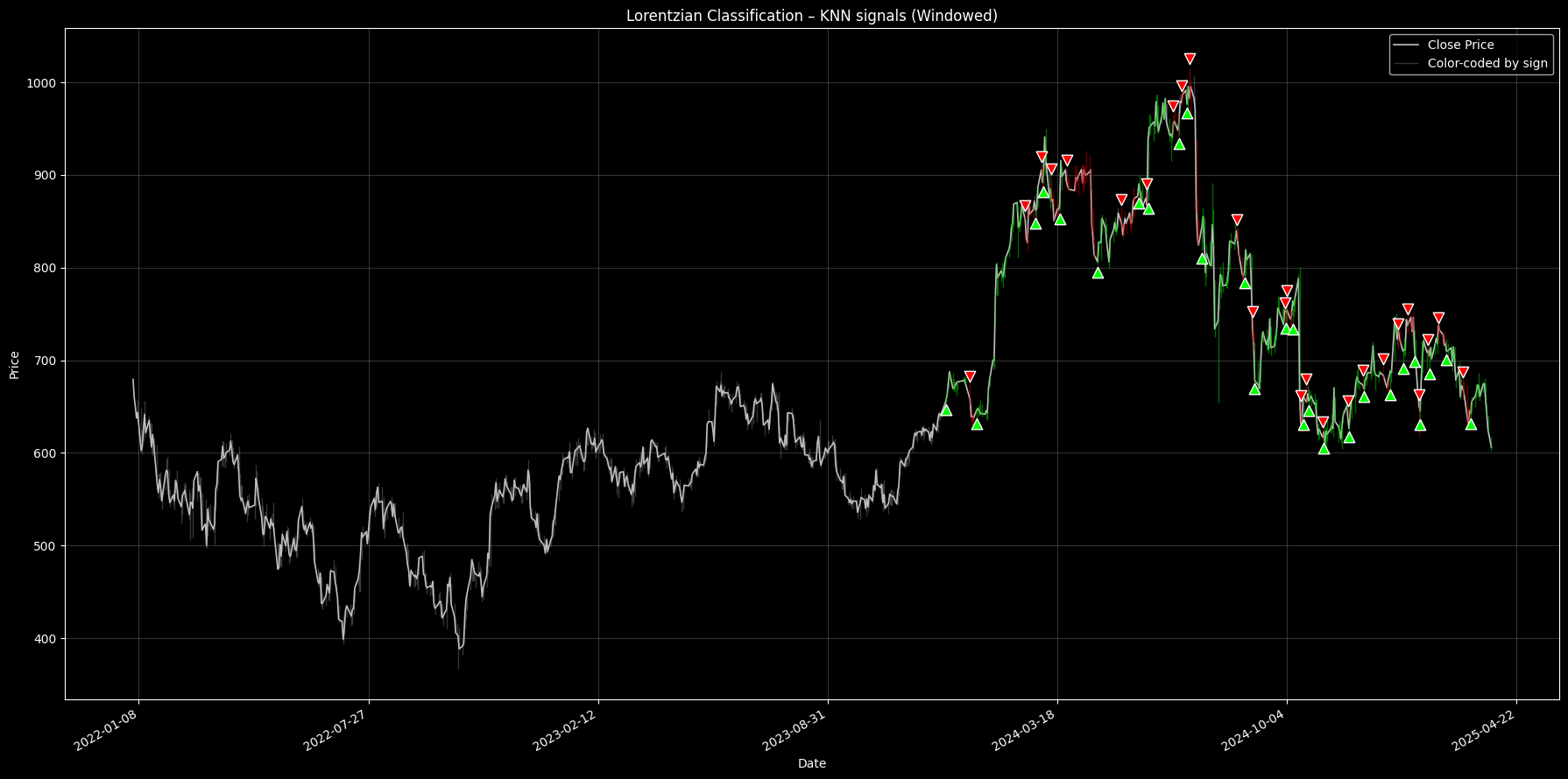
Figure 1. Stock Price chart with Lorentzian KNN signals. Vertical lines are color-coded by prediction strength (green = up, red = down, gray = neutral). Triangle markers show entry points based on signal transitions .
4. Discussion
4.1 Benefits
There are several advantages over traditional predictive models:
No model fitting: There’s nothing to train or optimize. Every prediction comes directly from historical patterns.
No overfitting risk: Since there’s no parameter tuning or target function, the method doesn’t conform to noise in the data.
Purely pattern-based: It relies on market memory, what the price action actually did in similar conditions, not forecasts or assumptions.
Intuitive and interpretable: You can inspect every signal. You know which past setups contributed to it, and how those played out. There’s no black box here.
4.2 Limitations and Improvements
There are some trade-offs:
No probability estimation: The output is a raw directional score, not a probability or confidence level.
Static logic: The method doesn’t adapt unless you manually adjust parameters (e.g. window size,
k, or lookahead). It treats all past data equally, which may not reflect evolving market regimes.
Possible improvements:
Weight neighbors by distance, so closer matches contribute more.
Cluster feature vectors before comparison to reduce noise.
Add a volatility filter to ignore low-conviction setups.
Explore alternate distance metrics (e.g. cosine similarity, Mahalanobis).