Big Tech Has Spent Billions Acquiring AI Smart Home Startups

The pattern is clear: when innovative companies successfully integrate AI into everyday products, tech giants pay billions to acquire them.

Google paid $3.2B for Nest.
Amazon spent $1.2B on Ring.
Generac spent $770M on EcoBee.

Now, a new AI-powered smart home company is following their exact path to acquisition—but is still available to everyday investors at just $1.90 per share.

With proprietary technology that connects window coverings to all major AI ecosystems, this startup has achieved what big tech wants most: seamless AI integration into daily home life.

Over 10 patents, 200% year-over-year growth, and a forecast to 5x revenue this year — this company is moving fast to seize the smart home opportunity.

The acquisition pattern is predictable. The opportunity to get in before it happens is not.

INVEST BEFORE BIG TECH MAKES THEIR MOVE

_{Past performance is not indicative of future results. Email may contain forward-looking statements. See US Offering for details. Informational purposes only.}

🚀 Your Investing Journey Just Got Better: Premium Subscriptions Are Here! 🚀

It’s been 4 months since we launched our premium subscription plans at GuruFinance Insights, and the results have been phenomenal! Now, we’re making it even better for you to take your investing game to the next level. Whether you’re just starting out or you’re a seasoned trader, our updated plans are designed to give you the tools, insights, and support you need to succeed.

Here’s what you’ll get as a premium member:

• Exclusive Trading Strategies: Unlock proven methods to maximize your returns.

• In-Depth Research Analysis: Stay ahead with insights from the latest market trends.

• Ad-Free Experience: Focus on what matters most—your investments.

• Monthly AMA Sessions: Get your questions answered by top industry experts.

• Coding Tutorials: Learn how to automate your trading strategies like a pro.

• Masterclasses & One-on-One Consultations: Elevate your skills with personalized guidance.

Our three tailored plans—Starter Investor, Pro Trader, and Elite Investor—are designed to fit your unique needs and goals. Whether you’re looking for foundational tools or advanced strategies, we’ve got you covered.

Don’t wait any longer to transform your investment strategy. The last 4 months have shown just how powerful these tools can be—now it’s your turn to experience the difference.

👉 Explore Premium Plans Now

Many traders tend to overcomplicate strategy testing by relying on advanced indicators, machine learning algorithms, and optimization techniques. But in reality, testing a profitable trading strategy can be simpler than most imagine.

In this guide, I’ll walk you through a straightforward method of identifying a real trading advantage using basic Python code. We’ll explore an intriguing market behavior triggered by institutional fund managers’ reporting practices.

The Hidden Edge: Window Dressing

Institutional fund managers often engage in a practice called “window dressing” at the end of the month. To make their performance appear stronger in monthly reports, they unload underperforming assets (like meme stocks) and buy more reliable investments (like bonds).

This creates a predictable market pattern:

• Buy bond ETFs at the end of the month when these managers make purchases

• Sell at the start of the following month as they rebalance their portfolios

Why is this edge still exploitable? Simply because it’s too small for the institutional players to concern themselves with, making it a great opportunity for individual traders to benefit from.

There’s a reason 400,000 professionals read this daily.

Join The AI Report, trusted by 400,000+ professionals at Google, Microsoft, and OpenAI. Get daily insights, tools, and strategies to master practical AI skills that drive results.

Sign up now for free and work smarter, not harder.

The Test: Validating the Hypothesis Using Basic Python

Let’s test this market edge using minimal Python code:

import pandas as pd
import numpy as np
import yfinance as yf

# Fetch historical data for TLT (Long-term Treasury Bond ETF)
data_tlt = yf.download("TLT", start="2002-01-01", end="2024-06-30")
data_tlt["log_return"] = np.log(data_tlt["Adj Close"] / data_tlt["Adj Close"].shift(1))

This segment pulls data for the TLT (a liquid bond ETF) and calculates log returns to keep our analysis precise.

Investigating the Pattern

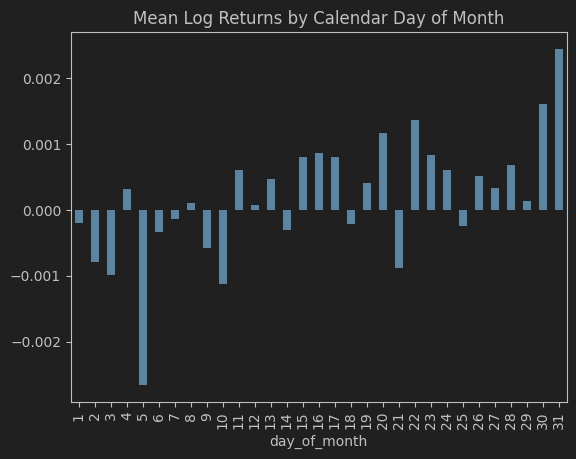
Next, let’s group returns based on each day of the calendar month:

data_tlt["day_of_month"] = data_tlt.index.day
data_tlt["year"] = data_tlt.index.year
daily_avg_returns = data_tlt.groupby("day_of_month").log_return.mean()
daily_avg_returns.plot.bar(title="Average Log Returns by Day of Month")

Upon reviewing the graph, we can observe that positive returns are more concentrated toward the end of the month, and negative returns appear at the beginning of the month.

Measuring the Strategy’s Effectiveness

Let’s compare the returns from the beginning and the end of each month:

# Initialize columns for first and last week's returns
data_tlt["first_week_returns"] = 0.0
data_tlt.loc[data_tlt.day_of_month <= 7, "first_week_returns"] = data_tlt[data_tlt.day_of_month <= 7].log_return

data_tlt["last_week_returns"] = 0.0
data_tlt.loc[data_tlt.day_of_month >= 23, "last_week_returns"] = data_tlt[data_tlt.day_of_month >= 23].log_return# Calculate the difference between last week's and first week's returns
data_tlt["last_week_less_first_week"] = data_tlt.last_week_returns - data_tlt.first_week_returns

This code creates a column showing the difference between the returns during the first week and the final week of each month.

Visualizing the Results

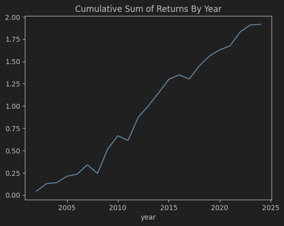
(data_tlt.groupby("year")
    .last_week_less_first_week.sum()
    .cumsum()
    .plot(title="Cumulative Monthly Strategy Returns By Year")
)

This graph highlights the cumulative returns from following our month-end strategy over time.

Why This Matters

This exercise underscores the following essential insights:

1. Profitable strategies don’t need to be overly complex.

2. Market inefficiencies (like the window dressing behavior) often present themselves in plain sight.

3. Simple Python code can quickly validate trading ideas.

Expanding the Search: Testing Multiple ETFs

We can extend the analysis by examining a variety of ETFs to see where this phenomenon is most pronounced.

# List of diverse ETFs to explore
etf_symbols = [
    "TLT",  # Long-term Treasury bonds
    "IEF",  # Intermediate Treasury bonds
    "SHY",  # Short-term Treasury bonds
    "LQD",  # Corporate bonds
    "HYG",  # High-yield bonds
    "AGG",  # Aggregate bonds
    "GLD",  # Gold
    "SPY",  # S&P 500
    "QQQ",  # Nasdaq 100
    "IWM"   # Russell 2000
]

We now perform a more extensive check across various asset classes.

Code to Calculate Strategy Returns Across Different ETFs

# Function to compute strategy performance for each ETF
def compute_etf_strategy_returns(symbol):
    try:
        # Download historical data
        df_etf = yf.download(symbol, start="2002-01-01", end="2024-06-30")
        
        # Calculate log returns
        df_etf["log_return"] = np.log(df_etf["Adj Close"] / df_etf["Adj Close"].shift(1))
        
        # Add day of the month
        df_etf["day_of_month"] = df_etf.index.day
        
        # Apply strategy: first and last week's returns
        df_etf["first_week_returns"] = 0.0
        df_etf.loc[df_etf.day_of_month <= 7, "first_week_returns"] = df_etf[df_etf.day_of_month <= 7].log_return
        
        df_etf["last_week_returns"] = 0.0
        df_etf.loc[df_etf.day_of_month >= 23, "last_week_returns"] = df_etf[df_etf.day_of_month >= 23].log_return
        
        # Calculate total strategy return and performance metrics
        strategy_return_total = (df_etf.last_week_returns - df_etf.first_week_returns).sum()
        strategy_return_annual = strategy_return_total / (len(df_etf) / 252)  # Annualized return
        strategy_sharpe = np.sqrt(252) * (df_etf.last_week_returns - df_etf.first_week_returns).mean() / (df_etf.last_week_returns - df_etf.first_week_returns).std()
        
        return {
            "symbol": symbol,
            "total_return": strategy_return_total,
            "annual_return": strategy_return_annual,
            "sharpe_ratio": strategy_sharpe
        }
    except Exception as e:
        print(f"Error processing {symbol}: {e}")
        return None

This function downloads each ETF’s data, applies our strategy, and returns the necessary performance metrics like total return, annual return, and Sharpe ratio.

Running the Strategy for All ETFs

# Analyze all ETFs in the list
analysis_results = []
for symbol in etf_symbols:
    result = compute_etf_strategy_returns(symbol)
    if result:
        analysis_results.append(result)

# Create a DataFrame to view performance metrics
results_df = pd.DataFrame(analysis_results)
results_df = results_df.sort_values("sharpe_ratio", ascending=False)# Format numerical results for clarity
results_df["total_return"] = results_df["total_return"].map("{:.2%}".format)
results_df["annual_return"] = results_df["annual_return"].map("{:.2%}".format)
results_df["sharpe_ratio"] = results_df["sharpe_ratio"].map("{:.2f}".format)# Display the results in a friendly format
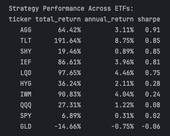
print("\nStrategy Performance Across ETFs:")
print(results_df.to_string(index=False))

Upon running this analysis, the results provide the following insights:

Key Findings

• Bond ETFs lead the performance with stronger Sharpe ratios and better returns, notably in AGG and TLT.

• The month-end effect is most pronounced in bond markets, aligning with the expectation that institutional managers would want to buy high-quality bonds to improve their portfolios.

• Gold (GLD) and equities such as SPY and QQQ show little to no advantage from the month-end pattern.

Strategy Optimization

Based on the results, you could:

• Concentrate efforts on bond ETFs such as AGG or TLT for a risk-adjusted return boost.

• Leverage the highest Sharpe ratio ETFs for enhanced profitability.

• Fine-tune your trading approach by adjusting exposure according to risk metrics or volatility.

Conclusion

This study shows that simple strategies can be extremely powerful. By keeping things straightforward, you can capitalize on under-the-radar market inefficiencies that others are overlooking.

Use this framework to adapt the strategy and test different ideas, such as expanding to alternative assets or adjusting based on seasonal trends. Often, the best strategies are the easiest ones, and they don’t require complex technologies to find.

You can save up to 100% on a Tradingview subscription with my refer-a-friend link. When you get there, click on the Tradingview icon on the top-left of the page to get to the free plan if that’s what you want.