CTV ads made easy: Black Friday edition
As with any digital ad campaign, the important thing is to reach streaming audiences who will convert. Roku’s self-service Ads Manager stands ready with powerful segmentation and targeting — plus creative upscaling tools that transform existing assets into CTV-ready video ads. Bonus: we’re gifting you $5K in ad credits when you spend your first $5K on Roku Ads Manager. Just sign up and use code GET5K. Terms apply.
🚀 Your Investing Journey Just Got Better: Premium Subscriptions Are Here! 🚀
It’s been 4 months since we launched our premium subscription plans at GuruFinance Insights, and the results have been phenomenal! Now, we’re making it even better for you to take your investing game to the next level. Whether you’re just starting out or you’re a seasoned trader, our updated plans are designed to give you the tools, insights, and support you need to succeed.
Here’s what you’ll get as a premium member:
Exclusive Trading Strategies: Unlock proven methods to maximize your returns.
In-Depth Research Analysis: Stay ahead with insights from the latest market trends.
Ad-Free Experience: Focus on what matters most—your investments.
Monthly AMA Sessions: Get your questions answered by top industry experts.
Coding Tutorials: Learn how to automate your trading strategies like a pro.
Masterclasses & One-on-One Consultations: Elevate your skills with personalized guidance.
Our three tailored plans—Starter Investor, Pro Trader, and Elite Investor—are designed to fit your unique needs and goals. Whether you’re looking for foundational tools or advanced strategies, we’ve got you covered.
Don’t wait any longer to transform your investment strategy. The last 4 months have shown just how powerful these tools can be—now it’s your turn to experience the difference.
Most traders use past price movements to estimate future trends. But options already embed those expectations and you can extract them.
Options prices not only reflect volatility. They capture the market’s collective expectations of future prices.
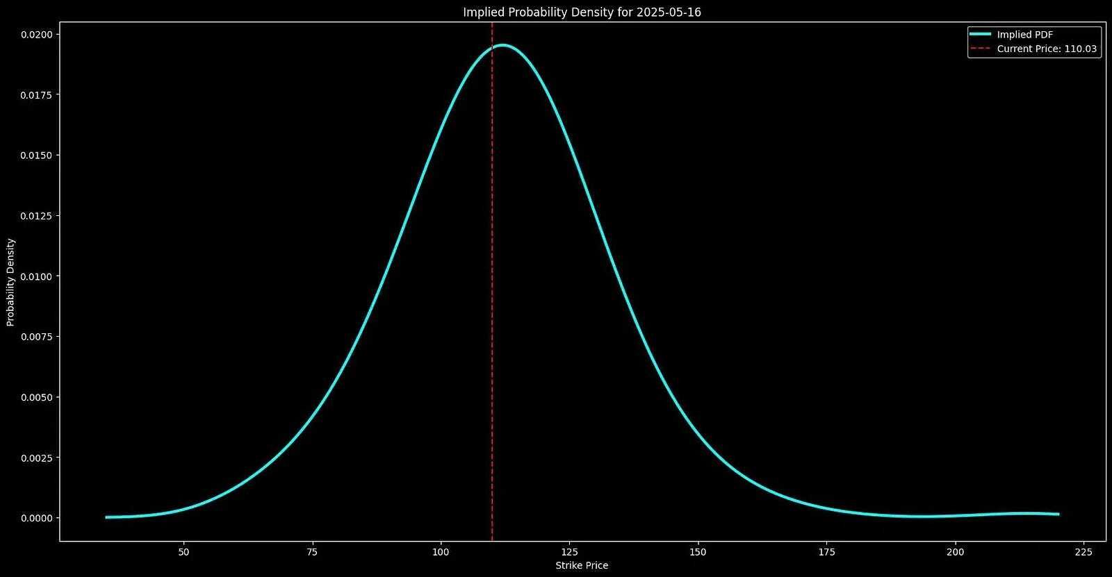
If we analyze option-implied probabilities, we can construct a forward-looking distribution of expected stock prices. We’ll do it in this article.
Specifically, we will construct a forward-looking distribution of expected stock prices based on option-implied probabilities for a given future date.
This approach goes beyond traditional indicators. It shows where traders believe a stock is most likely to end up by a given expiration date.
In this article, we’ll break down the step-by-step process of deriving market-implied probability distributions using options data.
The full end-to-end workflow is available in a Google Colab notebook, exclusively for paid subscribers of my newsletter. Paid subscribers also gain access to the complete article, including the full code snippet in the Google Colab notebook, which is accessible below the paywall at the end of the article. Subscribe now to unlock these benefits!
In this article, we’ll cover:
How to fetch and filter option chain data
Calculating implied volatility using the Black-Scholes model
Applying the Breeden-Litzenberger formula to extract risk-neutral probabilities
Smoothing the probability distribution for better insights
Visualizing a 3D implied probability surface over multiple expirations.
Business news as it should be.
Join 4M+ professionals who start their day with Morning Brew—the free newsletter that makes business news quick, clear, and actually enjoyable.
Each morning, it breaks down the biggest stories in business, tech, and finance with a touch of wit to keep things smart and interesting.
1. Extracting Market Expectations from Options
In a risk-neutral world, all assets are expected to grow at the risk-free rate. This assumption allows us to extract implied probabilities directly from option prices.
The core methodology behind our analysis is based on the Breeden-Litzenberger result.
It states that the second derivative of the call price with respect to the strike gives the risk-neutral probability density:

C is the call option price at strike K,
r is the risk-free rate,
T is the time to expiration.
This allows us to translate market prices directly into a probability distribution of future stock prices.
The Role Implied Volatility
Implied volatility, IV, represents market uncertainty about future price movements.
Unlike historical volatility, which looks backward, implied volatility is forward-looking. It reflects how risky traders expect a stock to be.
The Black-Scholes formula for pricing a European call option captures this:

d1 is

If we invert this formula, we can extract implied volatility from market prices and understand how uncertain traders are about the stock’s future.
Higher IV = wider probability distribution = greater uncertainty
Lower IV = narrower distribution = more confidence in price range
We now have the building blocks:
Option prices → Implied volatilities (market uncertainty)
Implied volatilities → Risk-neutral probabilities (expected future prices)
2. Setting Up the Data Pipeline
We can use yfinanceto extract option chain data for a particular ticker.
However, option chain data includes many contracts that are illiquid, and potentially mispriced. These should be filtered out.
Downloading Options Chain Data
Below, we fetch both the real-time option chain data for NVDAand its current stock price to compare it against the future expected market prices.
The first code snippet also includes all the necessary parameters for the functions that we will introduce later.
import yfinance as yf
import numpy as np
import pandas as pd
from datetime import datetime
from scipy.optimize import brentq
from scipy.stats import norm, gaussian_kde
from scipy.interpolate import splrep, BSpline
from scipy.integrate import simps
import plotly.graph_objects as go

# Ignore unnecessary warnings
import warnings
warnings.filterwarnings('ignore')


# Define parameters
ticker_symbol = "NVDA"
min_volume = 20         # Minimum volume for options liquidity
max_spread_ratio = 0.2  # Max acceptable bid-ask spread ratio

# Fetch the stock data
ticker = yf.Ticker(ticker_symbol)

# Get current stock price
current_price = ticker.history(period="1d")['Close'][-1]

# Get available expiration dates
expirations = ticker.options
print("Available Expiration Dates:", expirations)
Available Expiration Dates: ('2025-03-14', '2025-03-21', '2025-03-28', '2025-04-04', '2025-04-11', '2025-04-17', '2025-04-25', '2025-05-16', '2025-06-20', '2025-07-18', '2025-08-15', '2025-09-19', '2025-10-17', '2025-11-21', '2025-12-19', '2026-01-16', '2026-03-20', '2026-06-18', '2026-09-18', '2026-12-18', '2027-01-15', '2027-12-17')Select one expiration date (for example, the 8th in the list, i.e. ‘2025–05–16’ ) and fetch the call options data for that expiration.
# Select the nearest expiration date for demonstration
selected_expiry = ticker.options[7]

# Fetch call options data for this expiry
option_chain = ticker.option_chain(selected_expiry)
calls_df = option_chain.calls[['strike', 'lastPrice', 'bid', 'ask', 'volume']]

# Show initial raw data
calls_df.head()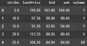
Figure 1. Raw option chain data before filtering. It shows strike prices, last traded prices, bid-ask quotes, and volume.
The data has a shape of (50, 5). However, many of these options are iliquid and will distort probability estimates. Only actively traded options are kept.
When AI Outperforms the S&P 500 by 28.5%
Did you catch these stocks?
Robinhood is up over 220% year to date.
Seagate is up 198.25% year to date.
Palantir is up 139.17% this year.
AltIndex’s AI model rated every one of these stocks as a “buy” before it took off.
The kicker? They use alternative data like reddit comments, congress trades, and hiring data.
We’ve teamed up with AltIndex to give our readers free access to their app for a limited time.
The next top performer is already taking shape. Will you be looking at the right data?
Past performance does not guarantee future results. Investing involves risk including possible loss of principal.
We define a function that removes options if:
Volume is too low (below a set threshold).
Bid price is zero (indicating no active buyers).
Bid-ask spread is too wide (poor liquidity).
# Function to filter out illiquid options
def filter_liquid_options(df, min_volume, max_spread_ratio):
    spread = df["ask"] - df["bid"]
    liquid_df = df[
        (df["volume"] >= min_volume) &
        (df["bid"] > 0) &
        ((spread := df["ask"] - df["bid"]) / df["ask"] <= max_spread_ratio)
    ]
    return liquid_df

# Apply filtering
filtered_calls_df = filter_liquid_options(calls_df, min_volume, max_spread_ratio)

# Display filtered data
filtered_calls_df.head()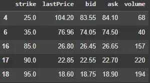
Figure 2. Filtered option chain data after removing illiquid contracts. It excludes options with low volume and wide bid-ask spreads.
The shape of the dataframe is now (25, 5). We continue the analysis with this dataframe.
3. Calculating Implied Volatility
As described, we calculate IV by inverting the Black-Scholes pricing model and solving for σ by numerically inverting this equation.
To find the IV that makes the Black-Scholes price match the observed market price, we use Brent’s method.
Brent’s algorithm finds roots of a function in a given interval. Brent’s method is a smart way to find where a function equals zero.
It combines two techniques:
The Secant Method (Fast but Risky) — It estimates the answer by drawing a straight line between two points and seeing where it crosses zero. This works well when the function behaves nicely, but it can sometimes jump too far.
The Bisection Method (Slow but Reliable) — It simply takes the middle point between two values and checks if the answer is there. This always works but takes more steps.
Brent’s method switches between these two approaches to get the best of both worlds — fast when possible, reliable when necessary.
Below, we calculate the IV and add it to the filtered_calls_df.
from scipy.optimize import brentq
from scipy.stats import norm


# Black-Scholes Call Option Pricing
def call_bs_price(S, K, T, r, sigma):
    if T <= 0:
        return max(S - K, 0)

    d1 = (np.log(S / K) + (r + 0.5 * sigma**2) * T) / (sigma * np.sqrt(T))
    d2 = d1 - sigma * np.sqrt(T)

    price = S * norm.cdf(d1) - K * np.exp(-r * T) * norm.cdf(d2)
    return price


# Function to calculate implied volatility
def implied_vol_call(price, S, K, T, r):
    if T <= 0:
        return np.nan

    def objective(sigma):
        return call_bs_price(S, K, T, r, sigma) - price

    try:
        implied_vol = brentq(objective, 1e-9, 5.0)
        return implied_vol
    except ValueError:
        return np.nan


# Define variables
T = (pd.to_datetime(selected_expiry) - pd.Timestamp.today()).days / 365.0
S = ticker.history().iloc[-1]['Close']
r = 0.04  # Risk-free rate (annualized)

# Calculate implied volatilities for all call options
filtered_calls_df['iv'] = filtered_calls_df.apply(
    lambda row: implied_vol_call(row['lastPrice'], S, row['strike'], T, r), axis=1
)

# Drop rows where implied volatility couldn't be calculated
filtered_calls_df.dropna(subset=['iv'], inplace=True)

# Check calculated implied volatilities
filtered_calls_df.head()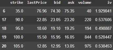
Figure 3. Option chain data with computed implied volatility. It includes IV values derived using the Black-Scholes model and Brent’s method.
4. Constructing the Risk-Neutral PDF
Once we have implied volatility for different strike prices, we can then extract a risk-neutral probability distribution of future stock prices.
Subscribe to our premium content to get access to the full article and code snippets.
Become a paying subscriber to get access to this post and other subscriber-only content.
Upgrade

