Find out why 1M+ professionals read Superhuman AI daily.

In 2 years you will be working for AI

Or an AI will be working for you

Here's how you can future-proof yourself:

1. Join the Superhuman AI newsletter – read by 1M+ people at top companies

2. Master AI tools, tutorials, and news in just 3 minutes a day

3. Become 10X more productive using AI

Join 1,000,000+ pros at companies like Google, Meta, and Amazon that are using AI to get ahead.

Sign up and start learning AI

🚀 Your Investing Journey Just Got Better: Premium Subscriptions Are Here! 🚀

It’s been 4 months since we launched our premium subscription plans at GuruFinance Insights, and the results have been phenomenal! Now, we’re making it even better for you to take your investing game to the next level. Whether you’re just starting out or you’re a seasoned trader, our updated plans are designed to give you the tools, insights, and support you need to succeed.

Here’s what you’ll get as a premium member:

• Exclusive Trading Strategies: Unlock proven methods to maximize your returns.

• In-Depth Research Analysis: Stay ahead with insights from the latest market trends.

• Ad-Free Experience: Focus on what matters most—your investments.

• Monthly AMA Sessions: Get your questions answered by top industry experts.

• Coding Tutorials: Learn how to automate your trading strategies like a pro.

• Masterclasses & One-on-One Consultations: Elevate your skills with personalized guidance.

Our three tailored plans—Starter Investor, Pro Trader, and Elite Investor—are designed to fit your unique needs and goals. Whether you’re looking for foundational tools or advanced strategies, we’ve got you covered.

Don’t wait any longer to transform your investment strategy. The last 4 months have shown just how powerful these tools can be—now it’s your turn to experience the difference.

👉 Explore Premium Plans Now

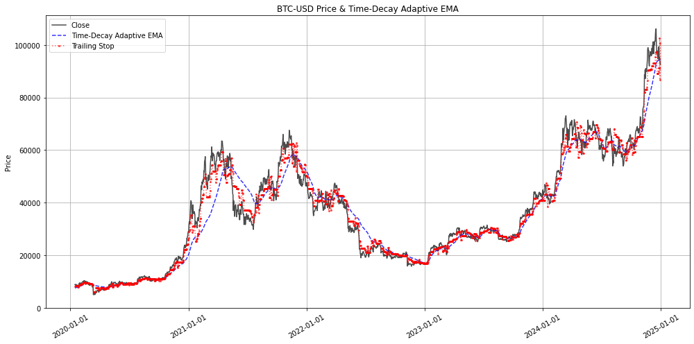
Traditional Exponential Moving Averages (EMAs) are a staple in technical analysis, but their fixed smoothing period can be a limitation in markets with dynamically changing volatility. The Time-Decay Adaptive Exponential Moving Average (TD-AEMA) addresses this by modulating its smoothing factor (α) based on an estimate of recent market noise, typically represented by an Exponentially Weighted Moving Average (EWMA) of historical volatility (σ). This article explores the construction, Python implementation, and analytical considerations of a trading strategy based on this adaptive filter.

Smarter Investing Starts with Smarter News

The Daily Upside helps 1M+ investors cut through the noise with expert insights. Get clear, concise, actually useful financial news. Smarter investing starts in your inbox—subscribe free.

Join 1M+ readers today.

Core Concepts: Volatility, Exponential Decay, and Adaptive Smoothing

1. The Adaptive Smoothing Factor (αₜ):
   The heart of the TD-AEMA lies in its adaptive smoothing factor, αₜ, which determines how much weight is given to the most recent price. It’s defined by the formula:

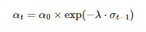
Where:

• α₀: This is a base (or maximum) smoothing factor. It represents the of the fastest desired EMA, corresponding to a minimum EMA period (Nₘᵢₙ), where α₀ = 2 / (Nₘᵢₙ + 1). This is the responsiveness the filter aims for when volatility is very low.

• σₜ₋₁: This is the EWMA of historical volatility from the previous period. It serves as our measure of current market “noise” or uncertainty.

• Historical volatility is first calculated (e.g., standard deviation of daily returns over a vol_calc_window).

• This raw volatility series is then smoothed using an EMA (with period vol_ema_period) to get σₜ.

• λ (lambda): This is a crucial decay rate or sensitivity parameter. It dictates how quickly the smoothing factor αₜ decreases (and thus the EMA slows down) as the EWMA volatility (σₜ₋₁) increases.

• A larger λ means αₜ will drop more sharply with rising volatility.

• A smaller λ makes αₜ less sensitive to volatility changes.

• The term exp(-λ.σₜ₋₁) acts as a dynamic scaling factor for α₀. As σₜ₋₁ increases, this exponential term decreases from 1 towards 0. Consequently, αₜ decreases from α₀ towards 0, resulting in a slower, more heavily smoothed EMA in higher volatility (noisier) conditions. This aligns with the goal of adapting to “changing noise.”

• The calculated αₜ can be optionally clipped to ensure it corresponds to an effective EMA period that doesn’t exceed a predefined maximum (e.g., period_ema_max_cap).

2. Time-Decay Adaptive EMA (TD-AEMA) Calculation:
With the adaptive αₜ determined for each day (based on the previous day’s EWMA volatility), the TD-AEMA is computed iteratively using the standard EMA formula:

3. Trading Strategy & Risk Management:

• A price crossover system with this TD-AEMA is used for signals.

• An ATR-based trailing stop loss and per-trade commissions are incorporated for a more realistic backtest.

Python Implementation Highlights

Let’s examine key code sections from the provided script.

Snippet 1: Calculating EWMA Volatility and the Adaptive Alpha

This snippet details how historical volatility is calculated, smoothed into an EWMA, and then used to derive the daily adaptive smoothing factor αₜ.

# --- Parameters (example for BTC-USD) ---
# vol_calc_window = 20         # Window for raw historical volatility
# vol_ema_period = 10          # Period for EWMA of historical volatility
# period_ema_min_for_alpha0 = 10 # Corresponds to alpha_0 (fastest EMA period)
# lambda_decay_param = 50.0      # Sensitivity of alpha decay to volatility
# period_ema_max_cap = 150       # Max effective period (min alpha)

# --- Column Names ---
# daily_return_col = "Daily_Return" (Assumed pre-calculated)
# hist_vol_col = f"HistVol_{vol_calc_window}d"
# ewma_vol_col = f"EWMA_Vol_{vol_ema_period}p"
# adaptive_alpha_col = "Adaptive_Alpha"

# --- Indicator Calculation (within pandas DataFrame 'df') ---

# 1. Historical Volatility (using daily standard deviation of returns)
df[hist_vol_col] = df[daily_return_col].rolling(window=vol_calc_window).std()

# 2. EWMA of Historical Volatility (our sigma_t)
df[ewma_vol_col] = df[hist_vol_col].ewm(span=vol_ema_period, adjust=False).mean()
# Fill initial NaNs for EWMA_Vol robustly
df[ewma_vol_col].fillna(method='bfill', inplace=True) 
df[ewma_vol_col].fillna(0, inplace=True) # If all are NaN (very short series), fill with 0

# 3. Calculate Adaptive Alpha (alpha_t)
alpha_0 = 2 / (period_ema_min_for_alpha0 + 1) # Base alpha for lowest volatility

# Alpha for today's EMA is based on YESTERDAY's EWMA_Vol
df[adaptive_alpha_col] = alpha_0 * np.exp(-lambda_decay_param * df[ewma_vol_col].shift(1))

# 4. Cap Alpha to correspond to a maximum EMA period (minimum alpha)
alpha_min_effective = 2 / (period_ema_max_cap + 1)
df[adaptive_alpha_col] = df[adaptive_alpha_col].clip(
    lower=alpha_min_effective, 
    upper=alpha_0 # Alpha cannot exceed alpha_0
)
# Fill initial NaNs for adaptive_alpha_col (e.g., from shift(1)) with alpha_0
df[adaptive_alpha_col].fillna(alpha_0, inplace=True) 

The adaptive_alpha_col now contains the daily smoothing factor for our TD-AEMA. The script also calculates an effective_period_col from this alpha for easier interpretation on plots.

Snippet 2: Iterative Calculation of the Time-Decay Adaptive EMA (TD-AEMA)

With the daily adaptive αₜ established, the TD-AEMA is computed day by day.

# --- Column Names ---
# adaptive_alpha_col = "Adaptive_Alpha" (calculated above)
# td_aema_filter_col = "TD_AEMA_Filter"

# --- Iterative TD-AEMA Calculation (within pandas DataFrame 'df') ---
df[td_aema_filter_col] = np.nan # Initialize column

# Seed the first TD-AEMA value (e.g., with the first close price where alpha is valid)
first_valid_alpha_idx = df[adaptive_alpha_col].first_valid_index()
if first_valid_alpha_idx is not None:
    df.loc[first_valid_alpha_idx, td_aema_filter_col] = df.loc[first_valid_alpha_idx, 'Close']
    
    start_loc_for_ema_loop = df.index.get_loc(first_valid_alpha_idx)

    for i_loop in range(start_loc_for_ema_loop + 1, len(df)):
        idx_today = df.index[i_loop]
        idx_prev = df.index[i_loop-1]
        
        # Alpha for today's EMA calculation is df.loc[idx_today, adaptive_alpha_col]
        # which was based on EWMA_Vol.shift(1)
        alpha_val = df.loc[idx_today, 'Alpha_Adaptive'] 
        current_close_val = df.loc[idx_today, 'Close']
        prev_filtered_price_val = df.loc[idx_prev, td_aema_filter_col]

        if any(pd.isna(val) for val in [alpha_val, current_close_val, prev_filtered_price_val]):
            df.loc[idx_today, td_aema_filter_col] = prev_filtered_price_val # Carry forward
        else:
            # Standard EMA formula with the dynamically changing alpha_val
            df.loc[idx_today, td_aema_filter_col] = alpha_val * current_close_val + (1 - alpha_val) * prev_filtered_price_val

# Fill any remaining NaNs at the start after loop
df[td_aema_filter_col].fillna(method='ffill', inplace=True)
df[td_aema_filter_col].fillna(method='bfill', inplace=True) 

This results in the td_aema_filter_col, our adaptive trendline.

Strategy Execution, Backtesting Framework, and Interpretation

The provided Python script (structured with a main run_time_decay_adaptive_ema_backtest function and a separate plotting function) then:

• Generates Trading Signals: Based on the previous day’s close crossing the previous day’s TD_AEMA_Filter. Trades are entered at the current day's open.

• Manages Risk: Uses an ATR-based trailing stop loss.

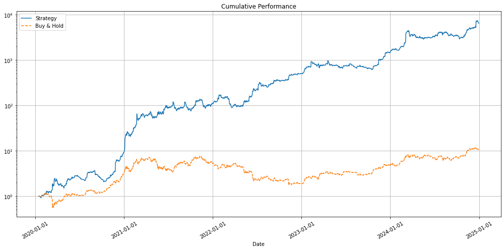
• Accounts for Costs: Deducts commission_bps_per_side.

• Calculates Performance Metrics: Cumulative return, annualized metrics, Sharpe ratio, max drawdown, and trade count are compared against a Buy & Hold benchmark.

Key Parameter Sensitivities (Research Focus):

• lambda_decay_param: This is highly critical. It controls the aggressiveness of the adaptation. Small changes can significantly alter how quickly the filter slows down.

• period_ema_min_for_alpha0: Sets the "fastest" state of the EMA.

• period_ema_max_cap: Prevents the filter from becoming excessively slow.

• Volatility Windows (vol_calc_window, vol_ema_period): These define how "recent" volatility is measured.

• ATR Stop Settings: As always, these affect trade duration and risk/reward.