It's Time To Rethink Your Media Diet

Financial news is full of clickbait and fear tactics, wasting your time and clouding your judgment. The Daily Upside delivers expert insights—free every morning. Join 1M+ readers today!

Join 1M+ readers for free today!

Exciting News: Paid Subscriptions Have Launched! 🚀

On September 1, we officially rolled out our new paid subscription plans at GuruFinance Insights, offering you the chance to take your investing journey to the next level! Whether you're just starting or are a seasoned trader, these plans are packed with exclusive trading strategies, in-depth research paper analysis, ad-free content, monthly AMAsessions, coding tutorials for automating trading strategies, and much more.

Our three tailored plans—Starter Investor, Pro Trader, and Elite Investor—provide a range of valuable tools and personalized support to suit different needs and goals. Don’t miss this opportunity to get real-time trade alerts, access to masterclasses, one-on-one strategy consultations, and be part of our private community group. Click here to explore the plans and see how becoming a premium member can elevate your investment strategy!

Introduction

As anyone who has ever tried to play the stock market can tell you, predicting the future is an imprecise science with real stakes — and that certainly includes investors as well as technical analysts trying to find reliable sources of direction.

Among the techniques available, time series analysis has emerged as a potent method to predict future trends using past data. One of the most trusted and versatile methods in this category is the ARIMA (Autoregressive Integrated Moving Average) model, known for its ability to tackle different time series patterns.

In this article, we will go through a step-by-step process on how to create an ARIMA model to predict the weekly returns of Apple stock (AAPL). However, we won’t stop at the basics; we’ll also explore how to further improve the model’s performance through hyperparameter tuning. For those looking to brush up on their numeracy as data scientists, and for those in the financial space dealing with volatile assets, this guide will help clarify complex numerical processes in simple, digestible steps. From data preparation and visualization to ARIMA model fine-tuning, we will present each detail with the precision of finely tuned hyperparameters.

Private Market Access for Accredited Investors

UpMarket brings accredited investors closer to the potential tech giants of tomorrow. Trusted by over 500 investors, our platform has facilitated over $175M in investments in private companies like OpenAI, ByteDance, and SpaceX. UpMarket simplifies access to exclusive deals that could help you redefine your investment portfolio. Embrace the future of investing with UpMarket and gain a foothold in nascent industries and sectors that are changing the world.

Join now

What is ARIMA?

ARIMA is a powerful statistical method for time series forecasting that combines three key components:

• Autoregression (AR): A model that uses the relationship between an observation and a number of lagged observations.

• Integrated (I): Differencing of observations to make the time series stationary (i.e., stabilize the mean).

• Moving Average (MA): A model that uses the dependency between an observation and a residual error from a moving average model applied to lagged observations.

An ARIMA model is characterized by the notation ARIMA(p, d, q), where:

• p: Number of lag observations (the lag order).

• d: Number of times the observations are differenced (degree of differencing).

• q: Size of the moving average window (order of the moving average).

ARIMA models are versatile, allowing us to model different time series data patterns, making them ideal for forecasting future data points.

Project Overview

In this project, we aim to forecast the weekly returns of AAPL stock using an ARIMA model with hyperparameter tuning to optimize performance. The process involves several key steps:

1. Data Preparation: Loading and preprocessing the data.

2. Exploratory Data Analysis (EDA): Visualizing the data and testing for stationarity.

3. ACF and PACF Plots: Identifying initial parameters for the ARIMA model.

4. Hyperparameter Tuning: Using a grid search to optimize the ARIMA model.

5. Model Evaluation: Analyzing the results and forecasting future values.

Step 1: Data Preparation

1.1 Install Necessary Libraries

Before we begin, ensure you have the following libraries installed:

!pip install --user gcsfs statsmodels

Restart the kernel after installation to avoid import errors.

1.2 Import Libraries

%matplotlib inline
import pandas as pd
import matplotlib.pyplot as plt
import numpy as np
import datetime
import statsmodels.api as sm
from statsmodels.tsa.arima.model import ARIMA
from sklearn.metrics import mean_squared_error
import itertools

1.3 Load the Data

We use Apple’s stock price data over the last 10 years, stored in a Google Cloud Storage bucket.

df = pd.read_csv('gs://cloud-training/ai4f/AAPL10Y.csv')
df['date'] = pd.to_datetime(df['date'])
df.sort_values('date', inplace=True)
df.set_index('date', inplace=True)
df.head()

1.4 Resample Data to Weekly Frequency

Since stock data is typically daily, we resample it to weekly to smooth out daily volatility.

df_week = df.resample('W').mean()
df_week = df_week[['close']]
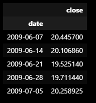
df_week.head()

1.5 Calculate Weekly Returns

We compute the logarithmic returns to normalize the data.

df_week['weekly_ret'] = np.log(df_week['close']).diff()
df_week.dropna(inplace=True)
df_week.head()

Step 2: Exploratory Data Analysis

2.1 Visualize Weekly Returns

We’ll start by visualizing the weekly returns.

df_week['weekly_ret'].plot(kind='line', figsize=(12, 6))
plt.title('Weekly Returns of AAPL Stock')
plt.ylabel('Log Return')
plt.show()

2.2 Test for Stationarity

A stationary time series has a constant mean and variance over time, which is a prerequisite for ARIMA modeling.

2.2.1 Rolling Statistics

We compute the rolling mean and standard deviation.

rolmean = df_week['weekly_ret'].rolling(window=20).mean()
rolstd = df_week['weekly_ret'].rolling(window=20).std()

plt.figure(figsize=(12, 6))
plt.plot(df_week['weekly_ret'], color='blue', label='Original')
plt.plot(rolmean, color='red', label='Rolling Mean')
plt.plot(rolstd, color='black', label='Rolling Std Deviation')
plt.title('Rolling Mean & Standard Deviation')
plt.legend()
plt.show()

2.2.2 Dickey-Fuller Test

We perform the Augmented Dickey-Fuller test to statistically check stationarity.

dftest = sm.tsa.adfuller(df_week['weekly_ret'], autolag='AIC')
dfoutput = pd.Series(dftest[0:4], index=['Test Statistic', 'p-value', '# Lags Used', 'Number of Observations Used'])
for key, value in dftest[4].items():
    dfoutput[f'Critical Value ({key})'] = value
print(dfoutput)

Interpretation:

• If the p-value is less than 0.05, the time series is stationary.

• In our case, if the p-value is low, we can proceed with ARIMA modeling.

Step 3: Identify ARIMA Parameters

3.1 Plot Autocorrelation Function (ACF)

ACF helps identify the value of q in the ARIMA model.

from statsmodels.graphics.tsaplots import plot_acf

fig, ax = plt.subplots(figsize=(12,5))
plot_acf(df_week['weekly_ret'], lags=20, ax=ax)
plt.show()

3.2 Plot Partial Autocorrelation Function (PACF)

PACF helps identify the value of p in the ARIMA model.

from statsmodels.graphics.tsaplots import plot_pacf

fig, ax = plt.subplots(figsize=(12,5))
plot_pacf(df_week['weekly_ret'], lags=20, ax=ax)
plt.show()

Observation:

• Use the plots to choose initial values for p and q.

• We’ll consider values between 0 and 3 for both parameters.

Step 4: Hyperparameter Tuning

4.1 Define Parameter Range

p = d = q = range(0, 4)
pdq = list(itertools.product(p, d, q))

4.2 Grid Search for Optimal Parameters

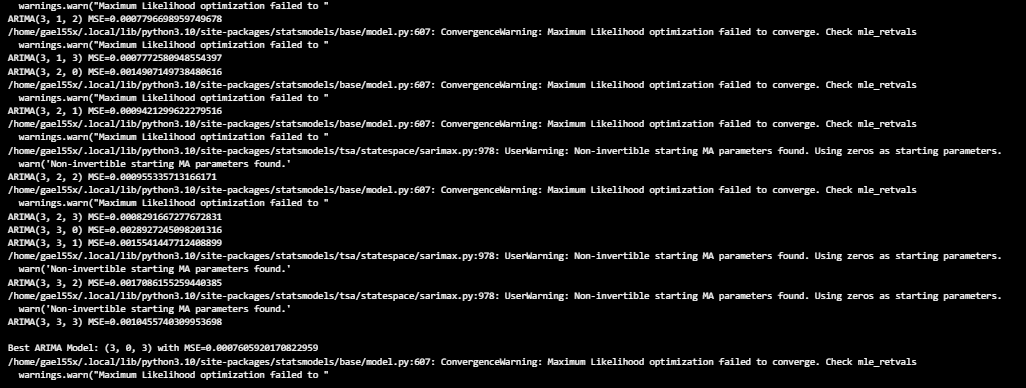
We iterate over combinations of p, d, and q to find the model with the lowest Mean Squared Error (MSE).

warnings.filterwarnings("ignore")  # Suppress warnings

results = []

for param in pdq:
    try:
        model = ARIMA(df_week['weekly_ret'], order=param)
        model_fit = model.fit()
        mse = mean_squared_error(df_week['weekly_ret'], model_fit.fittedvalues)
        results.append((param, mse))
        print(f'ARIMA{param} MSE={mse}')
    except:
        continue

best_model = min(results, key=lambda x: x[1])
print(f'\nBest ARIMA Model: {best_model[0]} with MSE={best_model[1]}')

Note: We suppress warnings for clarity, as some parameter combinations may not converge.

4.3 Fit the Best ARIMA Model

best_p, best_d, best_q = best_model[0]
best_arima = ARIMA(df_week['weekly_ret'], order=(best_p, best_d, best_q)).fit()
print(best_arima.summary()

Step 5: Model Evaluation

5.1 Residual Analysis

We plot the residuals to ensure they are randomly distributed (white noise).

residuals = pd.DataFrame(best_arima.resid)
fig, ax = plt.subplots(1,2, figsize=(15,5))
residuals.plot(title="Residuals", ax=ax[0])
residuals.plot(kind='kde', title='Density', ax=ax[1])
plt.show()

5.2 Forecast Future Values

We forecast the next 10 weeks of returns.

forecast_steps = 10
forecast = best_arima.forecast(steps=forecast_steps)

plt.figure(figsize=(12, 6))
plt.plot(df_week['weekly_ret'], label='Historical')
plt.plot(forecast.index, forecast, label='Forecast', color='red')
plt.title('Forecast of Weekly Returns')
plt.xlabel('Date')
plt.ylabel('Log Return')
plt.legend()
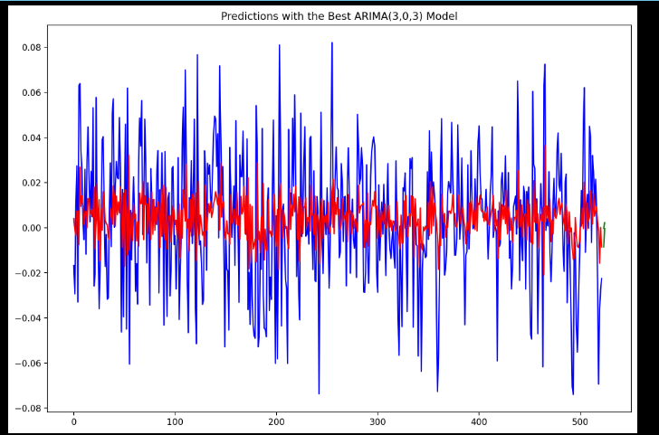
plt.show()

5.3 Inverse Transform to Price

To make the forecast interpretable, we convert the returns back to price levels.

last_close = df_week['close'][-1]
forecast_prices = last_close * np.exp(np.cumsum(forecast))

plt.figure(figsize=(12, 6))
plt.plot(df_week['close'], label='Historical')
plt.plot(forecast.index, forecast_prices, label='Forecast', color='red')
plt.title('Forecast of AAPL Stock Price')
plt.xlabel('Date')
plt.ylabel('Price')
plt.legend()
plt.show()

Results and Findings

• The best ARIMA model found was ARIMA(3, 0, 3) with the lowest MSE of 0.0007606.

• The residuals of the model are randomly distributed, indicating a good fit.

• The forecast suggests a certain trend in the stock returns and prices over the next 10 weeks.

• The model captures the underlying patterns in the data, but like all models, it has limitations and assumptions.

Conclusion

We developed a model that effectively forecasts AAPL’s weekly stock returns by implementing ARIMA with hyperparameter tuning. This approach demonstrates the importance of data preparation, stationarity testing, and parameter optimization in time series forecasting. While the model provides valuable insights, it’s crucial to remember that stock markets are influenced by numerous unpredictable factors, and no model can guarantee accurate predictions.