
In partnership with


Join 400,000+ executives and professionals who trust The AI Report for daily, practical AI updates.
Built for business—not engineers—this newsletter delivers expert prompts, real-world use cases, and decision-ready insights.
No hype. No jargon. Just results.
🚀 Your Investing Journey Just Got Better: Premium Subscriptions Are Here! 🚀
It’s been 4 months since we launched our premium subscription plans at GuruFinance Insights, and the results have been phenomenal! Now, we’re making it even better for you to take your investing game to the next level. Whether you’re just starting out or you’re a seasoned trader, our updated plans are designed to give you the tools, insights, and support you need to succeed.
Here’s what you’ll get as a premium member:
Exclusive Trading Strategies: Unlock proven methods to maximize your returns.
In-Depth Research Analysis: Stay ahead with insights from the latest market trends.
Ad-Free Experience: Focus on what matters most—your investments.
Monthly AMA Sessions: Get your questions answered by top industry experts.
Coding Tutorials: Learn how to automate your trading strategies like a pro.
Masterclasses & One-on-One Consultations: Elevate your skills with personalized guidance.
Our three tailored plans—Starter Investor, Pro Trader, and Elite Investor—are designed to fit your unique needs and goals. Whether you’re looking for foundational tools or advanced strategies, we’ve got you covered.
Don’t wait any longer to transform your investment strategy. The last 4 months have shown just how powerful these tools can be—now it’s your turn to experience the difference.

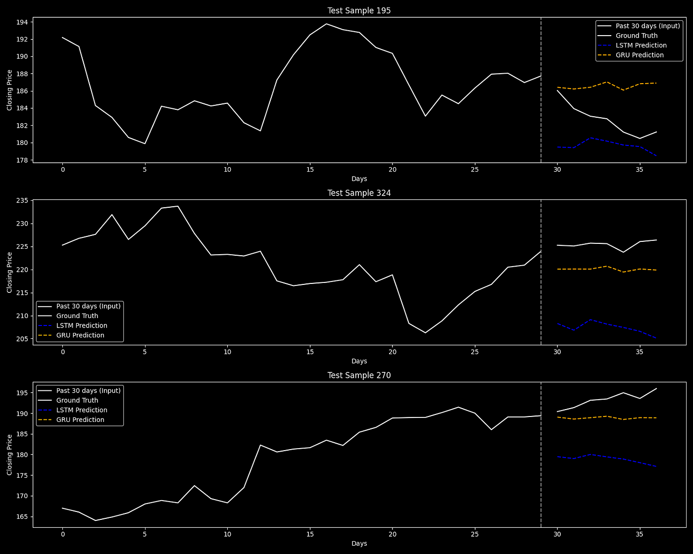
Comparison of LSTM and GRU model predictions against actual Apple stock closing prices over 7 days, following 30 days of historical data as input.
Stock prices move fast, but they rarely move without patterns.
If you could learn those patterns from history and forecast the next seven days, how useful would that be?
This article is a hands-on experiment using real historical data from Apple (AAPL) to test two of the most widely used deep learning models for time series forecasting — LSTM and GRU.
The goal is to see how well they can predict future closing prices based on past trends.
The Father-Son Duo Revolutionizing Homebuilding

Paolo and Galiano Tiramani founded BOXABL with a disruptive idea: bring factory efficiency to homebuilding. Today, new homes can roll off their assembly lines in ~4 hours – already building 700+. Now, they’re prepping for Phase 2, combining modules into larger townhomes, single-family homes, and apartments. And until 6/24, you can share in their growth.
*This is a paid advertisement for Boxabl’s Regulation A offering. Please read the offering circular at https://invest.boxabl.com/#circular
You’ll see:
How to collect and engineer features from raw stock data
How to structure the problem for sequence prediction
How each model is built, trained, and evaluated
A side-by-side comparison of results using real metrics and charts
Setup
We begin by installing and importing the necessary libraries:
!pip install yfinance scikit-learn matplotlib pandas numpy tensorflow tabulateimport yfinance as yf
import numpy as np
import pandas as pd
import matplotlib.pyplot as plt
from sklearn.preprocessing import MinMaxScaler
from sklearn.metrics import mean_squared_error, mean_absolute_error, r2_score
from tabulate import tabulate
from tensorflow.keras.models import Sequential
from tensorflow.keras.layers import LSTM, GRU, Dense, Dropout
import random
import os
# Ensure figure directory exists
os.makedirs("figures", exist_ok=True)
plt.style.use("dark_background")Data Collection and Feature Engineering
We’ll download historical stock data for Apple (AAPL) and engineer features commonly used in financial modeling.
# Download historical stock data
df = yf.download("AAPL", start="2015-01-01")
df.columns = df.columns.get_level_values(0)
df = df[['Close']]

# View the raw data
df.head()
We’ll then compute returns, moving averages, rolling standard deviation, and the Relative Strength Index (RSI). This is where you can engineer and include more features for more accurate predictions.
# Compute daily return
df["Return"] = df["Close"].pct_change()

# Moving averages and rolling statistics
df["MA7"] = df["Close"].rolling(window=7).mean()
df["MA21"] = df["Close"].rolling(window=21).mean()
df["STD21"] = df["Close"].rolling(window=21).std()

# RSI computation
delta = df["Close"].diff()
gain = np.where(delta > 0, delta, 0)
loss = np.where(delta < 0, -delta, 0)
gain = pd.Series(gain, index=df.index).rolling(window=14).mean()
loss = pd.Series(loss, index=df.index).rolling(window=14).mean()
rs = gain / loss
df["RSI"] = 100 - (100 / (1 + rs))

# Drop missing values
df.dropna(inplace=True)

# View the final dataframe
df.tail()
These features provide the model with more contextual information beyond just the price.
Sequence Generation
To train a deep learning model on time series, we convert the data into sequences of past values and their future targets.
def create_sequences(data, n_past=30, n_future=7):
    X, y = [], []
    for i in range(n_past, len(data) - n_future):
        X.append(data[i - n_past:i])
        y.append(data[i:i + n_future, 0])  # Predicting closing prices
    return np.array(X), np.array(y)

features = ["Close", "Return", "MA7", "MA21", "STD21", "RSI"]
scaler = MinMaxScaler()
scaled_data = scaler.fit_transform(df[features])

X, y = create_sequences(scaled_data, n_past=30, n_future=7)
split = int(0.8 * len(X))
X_train, y_train = X[:split], y[:split]
X_test, y_test = X[split:], y[split:]
Each input sequence spans 30 past days, and the model predicts the next 7 days of closing prices.
Visualizing Input and Target Sequences
Before training, we inspect a few training examples.
# Rescale the closing price back to original scale
close_index = features.index("Close")

def inverse_transform_close(data):
    dummy = np.zeros((len(data), len(features)))
    dummy[:, close_index] = data
    return scaler.inverse_transform(dummy)[:, close_index]

# Plot a few examples
num_examples = 3
plt.figure(figsize=(15, 4 * num_examples))

for i in range(num_examples):
    past = inverse_transform_close(X_train[i][:, close_index])
    future = inverse_transform_close(y_train[i])

    plt.subplot(num_examples, 1, i + 1)
    plt.plot(range(len(past)), past, label="Past 30 days", color="blue")
    plt.plot(range(len(past), len(past) + len(future)), future, label="Next 7 days", color="orange")
    plt.axvline(x=len(past) - 1, color="gray", linestyle="--")
    plt.title(f"Training Sample {i+1}")
    plt.xlabel("Days")
    plt.ylabel("Closing Price")
    plt.legend()

plt.tight_layout()
plt.savefig("figures/input_target_samples.png")
plt.show()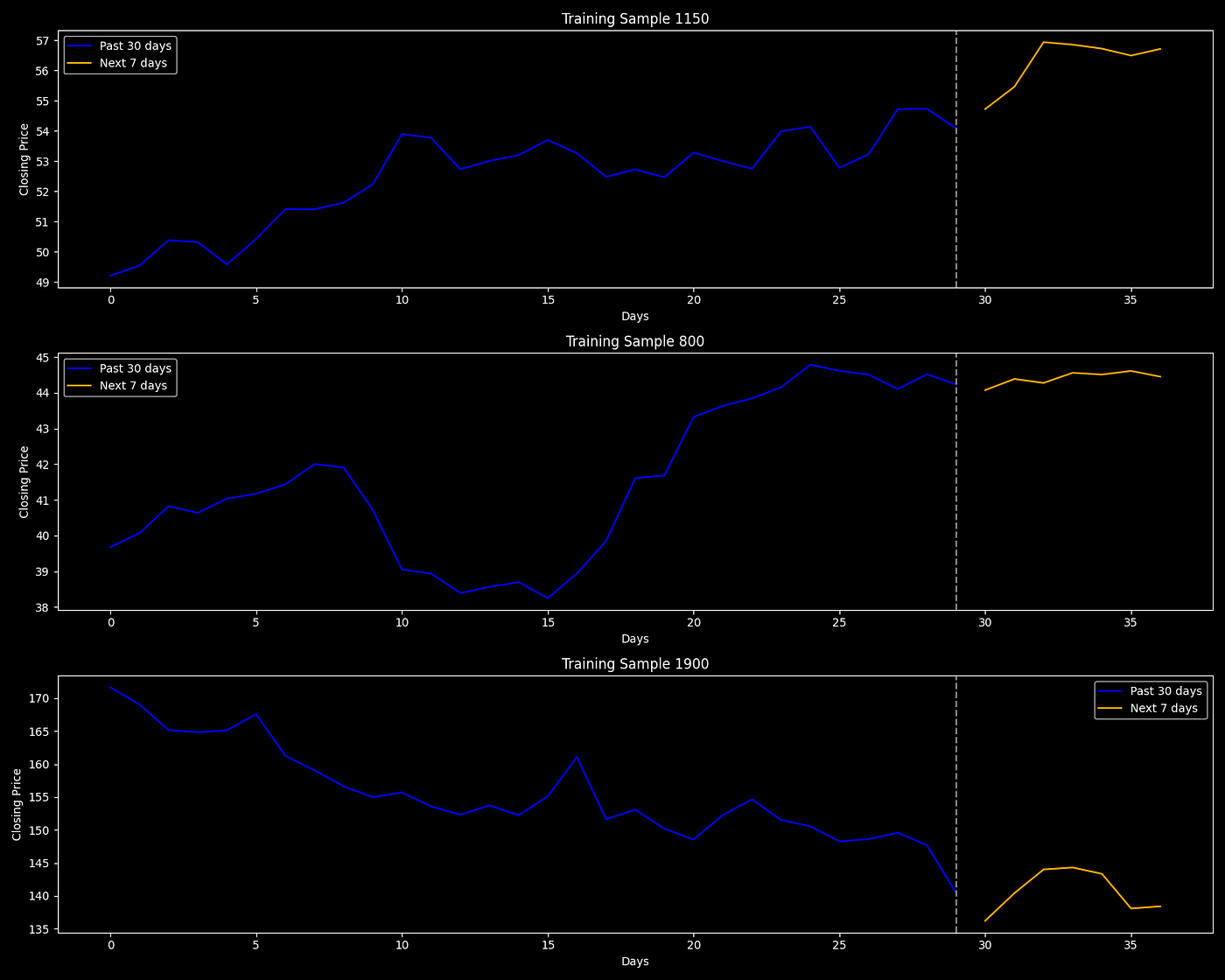
Sequence to Sequence Training Examples Chart
Model Building and Training
We train two separate models: one with an LSTM layer, and another with a GRU layer.
LSTM Model
def build_lstm(input_shape, output_steps):
    model = Sequential([
        LSTM(64, return_sequences=False, input_shape=input_shape),
        Dropout(0.2),
        Dense(output_steps)
    ])
    model.compile(optimizer="adam", loss="mse")
    return model

lstm_model = build_lstm(X_train.shape[1:], y_train.shape[1])
lstm_history = lstm_model.fit(
    X_train, y_train,
    validation_split=0.2,
    epochs=100,
    batch_size=32,
    verbose=1
)
GRU Model
def build_gru(input_shape, output_steps):
    model = Sequential([
        GRU(64, return_sequences=False, input_shape=input_shape),
        Dropout(0.2),
        Dense(output_steps)
    ])
    model.compile(optimizer="adam", loss="mse")
    return model

gru_model = build_gru(X_train.shape[1:], y_train.shape[1])
gru_history = gru_model.fit(
    X_train, y_train,
    validation_split=0.2,
    epochs=100,
    batch_size=32,
    verbose=1
)
Training Performance
def plot_history(history, model_name):
    plt.figure(figsize=(12, 6))
    plt.plot(history.history['loss'], label="Train Loss", color="blue")
    plt.plot(history.history['val_loss'], label="Val Loss", color="orange")
    plt.title(f"{model_name} Training History")
    plt.xlabel("Epochs")
    plt.ylabel("Loss")
    plt.legend()
    plt.savefig(f"figures/{model_name}_training_history.png")
    plt.show()
LSTM Training History
plot_history(lstm_history, "LSTM")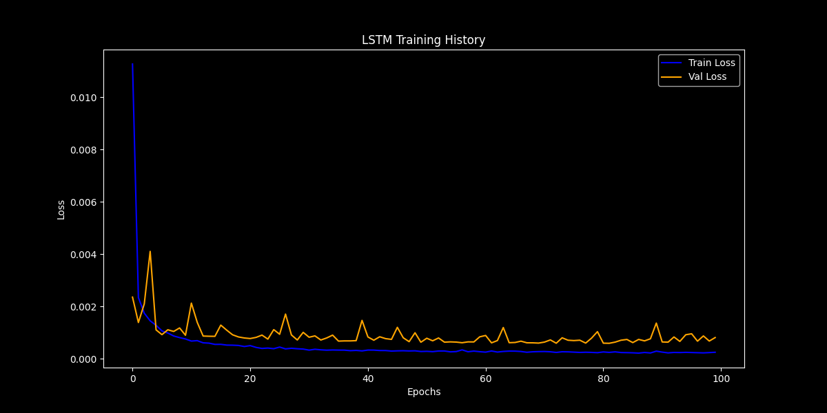
LSTM Training History
GRU Training History
plot_history(gru_history, "GRU")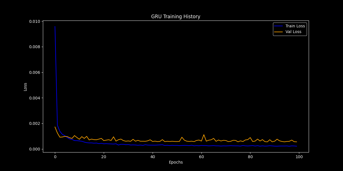
GRU Training History
These plots show how the training and validation loss evolved over time.
Model Evaluation
We generate predictions and evaluate the models on unseen data.
y_pred_lstm = lstm_model.predict(X_test)
y_pred_gru = gru_model.predict(X_test)

y_pred_lstm_inv = np.array([inverse_transform_close(seq) for seq in y_pred_lstm])
y_pred_gru_inv = np.array([inverse_transform_close(seq) for seq in y_pred_gru])
y_test_inv = np.array([inverse_transform_close(seq) for seq in y_test])
Define evaluation metrics:
def mean_absolute_percentage_error(y_true, y_pred):
    y_true, y_pred = np.array(y_true), np.array(y_pred)
    return np.mean(np.abs((y_true - y_pred) / y_true)) * 100

def evaluate_predictions(y_true, y_pred):
    y_true_flat = y_true.flatten()
    y_pred_flat = y_pred.flatten()

    mse = mean_squared_error(y_true_flat, y_pred_flat)
    mae = mean_absolute_error(y_true_flat, y_pred_flat)
    rmse = np.sqrt(mse)
    mape = mean_absolute_percentage_error(y_true_flat, y_pred_flat)
    r2 = r2_score(y_true_flat, y_pred_flat)

    return mse, mae, rmse, mape, r2

metrics_lstm = evaluate_predictions(y_test_inv, y_pred_lstm_inv)
metrics_gru  = evaluate_predictions(y_test_inv, y_pred_gru_inv)

headers = ["Model", "MSE", "MAE", "RMSE", "MAPE (%)", "R²"]
results = [
    ["LSTM"] + [round(m, 5) for m in metrics_lstm],
    ["GRU"]  + [round(m, 5) for m in metrics_gru]
]

print(tabulate(results, headers=headers, tablefmt="pretty"))
+-------+-----------+----------+----------+----------+---------+
| Model | MSE | MAE | RMSE | MAPE (%) | R² |
+-------+-----------+----------+----------+----------+---------+
| LSTM | 202.51944 | 11.83017 | 14.23093 | 5.64143 | 0.66759 |
| GRU | 52.45199 | 5.277 | 7.24237 | 2.59935 | 0.91391 |
+-------+-----------+----------+----------+----------+---------+Visualizing Random Predictions
Let’s visualize how both models perform on randomly selected samples from the test set.
num_examples = 3
plt.figure(figsize=(15, 4 * num_examples))

random_indices = random.sample(range(len(y_test)), num_examples)  # Pick random unique indices

for i, idx in enumerate(random_indices):
    past = inverse_transform_close(X_test[idx][:, close_index])  # Add this line to plot past input
    true = inverse_transform_close(y_test[idx])
    pred_lstm = inverse_transform_close(y_pred_lstm[idx])
    pred_gru = inverse_transform_close(y_pred_gru[idx])

    plt.subplot(num_examples, 1, i + 1)

    # Plot input sequence (past 30 days)
    plt.plot(range(len(past)), past, label="Past 30 days (Input)", color="white")

    # Plot predictions and ground truth (next 7 days)
    plt.plot(range(len(past), len(past) + len(true)), true, label="Ground Truth", color="white")
    plt.plot(range(len(past), len(past) + len(pred_lstm)), pred_lstm, label="LSTM Prediction", linestyle="--", color="blue")
    plt.plot(range(len(past), len(past) + len(pred_gru)), pred_gru, label="GRU Prediction", linestyle="--", color="orange")

    plt.axvline(x=len(past) - 1, color="gray", linestyle="--")
    plt.title(f"Test Sample {idx}")
    plt.xlabel("Days")
    plt.ylabel("Closing Price")
    plt.legend()

plt.tight_layout()
plt.savefig("figures/predictions_vs_ground_truth.png")
plt.show()
Models Predictions with Ground Truth Data
These visualizations help us understand how each model tracks actual market movement over a one-week horizon.
The GRU model outperformed the LSTM across all metrics, with lower error rates and stronger predictive accuracy.
Its ability to capture short-term patterns in Apple’s stock price was more consistent and precise.
This shows how small architectural changes in deep learning can lead to meaningful improvements.
You can build on this by testing other stocks, adding new features, or incorporating market signals like news or volume.
This notebook offers a simple yet powerful starting point for stock price forecasting with deep learning.