Lawmaker stock trades can now be copied automatically on Dub

On Dub, you don't pick stocks. You pick the people you want to copy, with portfolios based on hedge fund managers, investing experts, and even law makers.

Portfolios are automatically adjusted with quantitative investment strategies based on multiple factors around a long-term strategy, aiming to have high performance despite disclosure delays.

Dub is SEC-registered, member FINRA. All deposits are SIPC-insured.

Free Trial, $89 annually (iOS)

Not investment advice. Full disclosures here

Exciting News: Paid Subscriptions Have Launched! 🚀

On September 1, we officially rolled out our new paid subscription plans at GuruFinance Insights, offering you the chance to take your investing journey to the next level! Whether you're just starting or are a seasoned trader, these plans are packed with exclusive trading strategies, in-depth research paper analysis, ad-free content, monthly AMAsessions, coding tutorials for automating trading strategies, and much more.

Our three tailored plans—Starter Investor, Pro Trader, and Elite Investor—provide a range of valuable tools and personalized support to suit different needs and goals. Don’t miss this opportunity to get real-time trade alerts, access to masterclasses, one-on-one strategy consultations, and be part of our private community group. Click here to explore the plans and see how becoming a premium member can elevate your investment strategy!

In this article, I’ll walk you through how I combined mean reversion theory with LSTM neural networks to create a trading strategy that, over two years, turned an investment of $500 into $800. We will be discussing data preprocessing, model training, strategy implementation, and performance evaluation, thus avoiding the leakage of data and using effective risk management.

Understanding Mean Reversion

Mean Reversion is a financial strategy that indicates that asset prices tend to move towards their historical mean over time. Market players utilize this strategy in the following ways:

• Buying assets when the prices are below the mean.

• Selling when prices exceed the mean.

This strategy assumes that deviations from the mean are temporary, and prices will return to their average over time (Poterba & Summers, 1988). This phenomenon has been observed across various markets and asset classes (Balvers et al., 2000).

2 Cards Charging 0% Interest Until 2026

Paying down your credit card balance can be tough with the majority of your payment going to interest. Avoid interest charges for up to 18 months with these cards.

Learn more

The Role of LSTMs

Long Short-Term Memory (LSTM) networks are sequence-specific neural networks designed for sequential data, like time-series financial data (Hochreiter & Schmidhuber, 1997). They excel at identifying patterns and predicting future price movements by “remembering” long-term dependencies in data. Previous studies have demonstrated the effectiveness of LSTMs in predicting financial market trends (Fischer & Krauss, 2018; Bao et al., 2017).

By pairing LSTMs with mean reversion, we can create a predictive edge that enhances the profitability potential of this strategy.

Import Libraries

We import libraries for data retrieval (yfinance), data manipulation (pandas, numpy), visualization (matplotlib, mplfinance), preprocessing and evaluation (sklearn), and building neural networks (tensorflow, keras). We suppress warnings for cleaner output.

import yfinance as yf
import pandas as pd
import numpy as np
import matplotlib.pyplot as plt
%matplotlib inline
from sklearn.preprocessing import StandardScaler
from sklearn.metrics import mean_squared_error, mean_absolute_error
import tensorflow as tf
from tensorflow.keras.models import Sequential
from tensorflow.keras.layers import LSTM, Dense, Dropout
from tensorflow.keras.callbacks import EarlyStopping
from tensorflow.keras.regularizers import l2
import mplfinance as mpf  # For candlestick plotting
import warnings
warnings.filterwarnings("ignore")

import os
os.environ['TF_CPP_MIN_LOG_LEVEL'] = '2'

Download Cryptocurrency Data

Then, we fetch daily price data for Bitcoin over the past seven years, ensuring we have sufficient historical data for our model.

import datetime

ticker = 'BTC-USD'

end_date = datetime.datetime.now()

# set start_date 7 years back
start_date = end_date - datetime.timedelta(days=7*365)

start_date_str = start_date.strftime('%Y-%m-%d')
end_date_str = end_date.strftime('%Y-%m-%d')

# download data using yfinance with daily intervals
data = yf.download(
    tickers=ticker,
    start=start_date_str,
    end=end_date_str,
    interval='1d'
)
data.dropna(inplace=True)

if data.empty:
    raise ValueError("No data downloaded. Please check the ticker symbol and internet connection.")
else:
    print("Data downloaded successfully.")

At this stage, the dataset includes columns like Open, High, Low, Close, Adjusted Close, and Volume.

Data Preprocessing

To prepare the data for the LSTM model, we calculate several technical indicators that capture price trends and volatility.

if 'Close' in data.columns:
    # calculating moving averages
    data['MA20'] = data['Close'].rolling(window=20).mean()
    data['MA50'] = data['Close'].rolling(window=50).mean()

    # calculating Bollinger Bands
    data['STD'] = data['Close'].rolling(window=20).std()
    data['Upper_Band'] = data['MA20'] + (data['STD'] * 2.5)
    data['Lower_Band'] = data['MA20'] - (data['STD'] * 2.5)

    # calculating %B (Bollinger Band %)
    data['%B'] = (data['Close'] - data['Lower_Band']) / (data['Upper_Band'] - data['Lower_Band'])

    # calculating RSI
    delta = data['Close'].diff()
    up = delta.clip(lower=0)
    down = -1 * delta.clip(upper=0)
    roll_up = up.rolling(14).mean()
    roll_down = down.rolling(14).mean()
    RS = roll_up / roll_down
    data['RSI'] = 100.0 - (100.0 / (1.0 + RS))

    # calculating MACD and Signal Line
    exp1 = data['Close'].ewm(span=12, adjust=False).mean()
    exp2 = data['Close'].ewm(span=26, adjust=False).mean()
    data['MACD'] = exp1 - exp2
    data['Signal_Line'] = data['MACD'].ewm(span=9, adjust=False).mean()

    # calculating Momentum
    data['Momentum'] = data['Close'] - data['Close'].shift(10)

    # calculating Average True Range (ATR)
    data['TR'] = data[['High', 'Close']].max(axis=1) - data[['Low', 'Close']].min(axis=1)
    data['ATR'] = data['TR'].rolling(window=14).mean()

    # drop rows if they have NaN values
    data.dropna(inplace=True)
else:
    raise ValueError("The 'Close' column is missing from the data.")

We calculate technical indicators such as Moving Averages, Bollinger Bands, RSI, MACD, Momentum, and ATR. These indicators help capture trends, momentum, and volatility, which are essential for price prediction and signal generation.

Visualizing Technical Indicators

Let’s visualize some of these indicators.

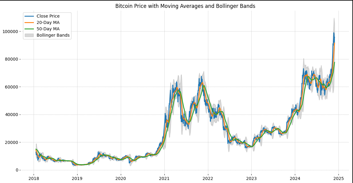
• The plot shows the closing price of Bitcoin along with the 20-day and 50-day moving averages, and Bollinger Bands. This helps visualize the price trends and volatility.

Preparing the Data for the LSTM

We scale the data and create sequences for the LSTM model.

features = ['Close', '%B', 'RSI', 'MACD', 'Signal_Line', 'Momentum', 'ATR']

# feature scaling 
scaler = StandardScaler()
scaled_data = scaler.fit_transform(data[features])

def create_sequences(data, seq_length):
    X = []
    y = []
    for i in range(seq_length, len(data)):
        X.append(data[i - seq_length:i])
        y.append(data[i, 0])  
    return np.array(X), np.array(y)


seq_length = 60 

X, y = create_sequences(scaled_data, seq_length)

if X.size == 0 or y.size == 0:
    raise ValueError("Insufficient data to create sequences. Try reducing the sequence length.")

We use a sequence length of 60 days to capture two months of historical data for each prediction, balancing sufficient historical context with computational efficiency.

Splitting Data into Training and Testing Sets

We split the data into training (5 years) and testing (2 years) sets, ensuring no data leakage occurs.

train_size = int(5 * 365)  # 5 years for training
test_size = int(2 * 365)   # 2 years for testing

X_train = X[:train_size]
y_train = y[:train_size]
X_test = X[train_size:train_size + test_size]
y_test = y[train_size:train_size + test_size]

• By splitting the data into 5 years for training and 2 years for testing, we ensure that our model is trained on past data and tested on future data, avoiding data leakage.

Building and Training the LSTM Model

The model is built with stacked LSTM layers and dropout for regularization.

model = Sequential()
model.add(LSTM(units=128, return_sequences=True, input_shape=(X_train.shape[1], X_train.shape[2]), kernel_regularizer=l2(0.001)))
model.add(Dropout(0.3))
model.add(LSTM(units=64, return_sequences=False, kernel_regularizer=l2(0.001)))
model.add(Dropout(0.3))
model.add(Dense(1))

model.compile(optimizer='adam', loss='mean_squared_error')

# early Stopping
early_stopping = EarlyStopping(monitor='val_loss', patience=5)

history = model.fit(
    X_train,
    y_train,
    epochs=100,
    batch_size=32,
    validation_data=(X_test, y_test),
    callbacks=[early_stopping]
)

Our model starts with an LSTM layer with 128 units and L2 regularization to prevent overfitting. We apply dropout with a rate of 0.3 for regularization. A second LSTM layer with 64 units follows, capturing more abstract patterns. Finally, we have a dense layer to produce the output.

Make Predictions and Evaluate the Model

We make predictions on the test set and evaluate the model’s performance using MAE, MSE, and RMSE.

predictions = model.predict(X_test)

# error metrics
mae = mean_absolute_error(y_test, predictions)
mse = mean_squared_error(y_test, predictions)
rmse = np.sqrt(mse)

print(f"MAE: {mae}")
print(f"MSE: {mse}")
print(f"RMSE: {rmse}")

# transform predictions and actual values
zeros = np.zeros((predictions.shape[0], len(features) - 1))
predictions_extended = np.hstack((predictions, zeros))
actuals_extended = np.hstack((y_test.reshape(-1, 1), zeros))

# use inverse transform function from the scaler
predicted_close = scaler.inverse_transform(predictions_extended)[:, 0]
actual_close = scaler.inverse_transform(actuals_extended)[:, 0]

# Plot Predicted vs Actual Close Prices
plt.figure(figsize=(12, 6))
plt.plot(actual_close, label='Actual Close Price')
plt.plot(predicted_close, label='Predicted Close Price')
plt.title('Predicted vs Actual Close Prices')
plt.xlabel('Time')
plt.ylabel('Price (USD)')
plt.legend()
plt.show()

Results:
MAE: 0.1483047224232923
MSE: 0.04917100263081512
RMSE: 0.22174535537596976

• The model achieved a Mean Absolute Error (MAE) of 0.1483 and a Root Mean Squared Error (RMSE) of 0.2217 on the test set, indicating reasonable predictive performance.

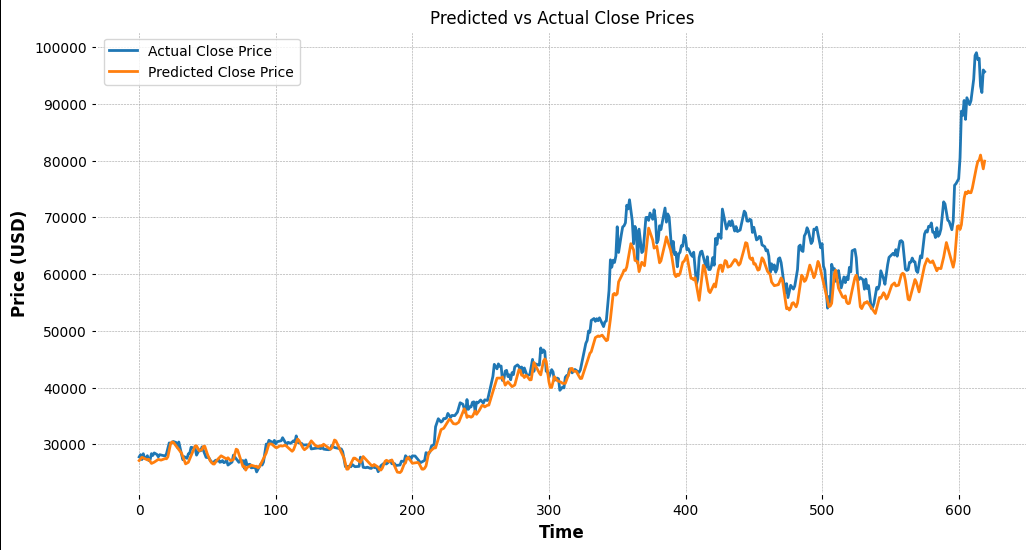
• We also transform the predictions back to the original scale.

Implement the Trading Strategy

We implement a mean reversion trading strategy based on the model’s predictions and technical indicators.

test_data = data.iloc[train_size + seq_length:train_size + seq_length + test_size].copy()
test_data['Predicted_Close'] = predicted_close
test_data['Actual_Close'] = actual_close

# predicted changes calculations
test_data['Predicted_Change'] = (test_data['Predicted_Close'] - test_data['Actual_Close']) / test_data['Actual_Close']

# genereate trading signals based on adjusted strategy
test_data['Signal'] = 0

# adjust thresholds based on percentiles
rsi_buy_threshold = test_data['RSI'].quantile(0.4)
rsi_sell_threshold = test_data['RSI'].quantile(0.6)
predicted_change_buy_threshold = test_data['Predicted_Change'].quantile(0.6)
predicted_change_sell_threshold = test_data['Predicted_Change'].quantile(0.4)

# buy signal
test_data.loc[
    (test_data['Predicted_Change'] > predicted_change_buy_threshold) &
    (test_data['RSI'] < rsi_buy_threshold),
    'Signal'
] = 1

# sell signal
test_data.loc[
    (test_data['Predicted_Change'] < predicted_change_sell_threshold) &
    (test_data['RSI'] > rsi_sell_threshold),
    'Signal'
] = -1

# count the number of buy and sell signals
num_buy_signals = (test_data['Signal'] == 1).sum()
num_sell_signals = (test_data['Signal'] == -1).sum()

print(f"Number of Buy Signals: {num_buy_signals}")
print(f"Number of Sell Signals: {num_sell_signals}")

• Our strategy generated 133 buy signals and 142 sell signals over the test period. This suggests that the model identified several opportunities where the asset was undervalued or overvalued relative to its predicted mean.

Simulate Trading with Risk Management

We simulate trading with an initial capital of $500, incorporating transaction costs, stop-loss, and take-profit mechanisms.

initial_capital = 500.0
positions = []
cash = initial_capital
holdings = 0
portfolio_value = []
transaction_cost = 0.0005  # let's assume 0.05% trading fee per trade
stop_loss_percent = 0.1    # 10% stop-loss
take_profit_percent = 0.2  # 20% take-profit
entry_price = None

for index, row in test_data.iterrows():
    price = row['Actual_Close']
    signal = row['Signal']
    if signal == 1 and cash > 0:
        # buy with a portion of cash (e.g., 50%)
        amount_to_buy = (cash * 0.5) * (1 - transaction_cost)
        holdings += amount_to_buy / price
        cash -= amount_to_buy
        entry_price = price
        positions.append({'Date': index, 'Position': 'Buy', 'Price': price})
    elif signal == -1 and holdings > 0:
        # sell all holdings
        amount_to_sell = holdings * price * (1 - transaction_cost)
        cash += amount_to_sell
        holdings = 0
        entry_price = None
        positions.append({'Date': index, 'Position': 'Sell', 'Price': price})
    elif holdings > 0:
        # check for stop-loss or take-profit
        if price <= entry_price * (1 - stop_loss_percent):
            # trigger stop-loss
            amount_to_sell = holdings * price * (1 - transaction_cost)
            cash += amount_to_sell
            holdings = 0
            positions.append({'Date': index, 'Position': 'Stop Loss Sell', 'Price': price})
            entry_price = None
        elif price >= entry_price * (1 + take_profit_percent):
            # trigger take-profit
            amount_to_sell = holdings * price * (1 - transaction_cost)
            cash += amount_to_sell
            holdings = 0
            positions.append({'Date': index, 'Position': 'Take Profit Sell', 'Price': price})
            entry_price = None
    total_value = cash + holdings * price
    portfolio_value.append(total_value)

# musst ensure portfolio_value matches test_data length
test_data['Portfolio_Value'] = portfolio_value[:len(test_data)]

We simulate trades by executing buy and sell orders based on the generated signals, while applying transaction costs, stop-loss, and take-profit rules.

Calculate Performance Metrics

We calculate key performance metrics to evaluate the strategy’s effectiveness.

# calculate daily returns and cumulative returns
test_data['Daily_Return'] = test_data['Portfolio_Value'].pct_change()
test_data['Cumulative_Return'] = (1 + test_data['Daily_Return']).cumprod()

# calculate annualized return
total_days = (test_data.index[-1] - test_data.index[0]).days
if total_days == 0:
    total_days = 1  # Avoid division by zero

annualized_return = (test_data['Cumulative_Return'].iloc[-1]) ** (365 / total_days) - 1

# calculate Sharpe Ratio
returns = test_data['Daily_Return'].dropna()
if returns.std() != 0:
    sharpe_ratio = (returns.mean() / returns.std()) * np.sqrt(252)  # Annualized Sharpe Ratio
else:
    sharpe_ratio = 0.0

# calculate Max Drawdown
rolling_max = test_data['Portfolio_Value'].cummax()
drawdown = test_data['Portfolio_Value'] / rolling_max - 1
max_drawdown = drawdown.min()

# Print performance metrics
total_return = ((test_data['Portfolio_Value'].iloc[-1] - initial_capital) / initial_capital) * 100
print(f"Total Return: {total_return:.2f}%")
print(f"Annualized Return: {annualized_return * 100:.2f}%")
print(f"Sharpe Ratio: {sharpe_ratio:.2f}")
print(f"Max Drawdown: {max_drawdown * 100:.2f}%")

• Our strategy achieved a total return of 60.20% over the two-year test period, growing the initial $500 to approximately $800. The annualized return is 32.09%, which is significant. A Sharpe Ratio of 0.94 indicates a good return relative to the risk taken. The maximum drawdown of -16.88% shows the largest peak-to-trough decline during the period, which is acceptable given the returns.

Visualize Trading Signals

We plot buy and sell signals on a candlestick chart for better visualization.

# candlestick plotting
plot_data = data.loc[test_data.index][['Open', 'High', 'Low', 'Close']].copy()
plot_data.index.name = 'Date'

# buy and sell signal markers for plotting
buy_signals = test_data[test_data['Signal'] == 1]
sell_signals = test_data[test_data['Signal'] == -1]

# additional plots for buy and sell signals
apds = []

if not buy_signals.empty:
    buy_prices = data.loc[buy_signals.index, 'Close']
    buy_signals_plot = pd.DataFrame({'Price': buy_prices.values}, index=buy_signals.index)
    buy_signals_plot = buy_signals_plot.reindex(plot_data.index)
    apds.append(
        mpf.make_addplot(
            buy_signals_plot['Price'],
            type='scatter',
            markersize=100,
            marker='^',
            color='g'
        )
    )

if not sell_signals.empty:
    sell_prices = data.loc[sell_signals.index, 'Close']
    sell_signals_plot = pd.DataFrame({'Price': sell_prices.values}, index=sell_signals.index)
    sell_signals_plot = sell_signals_plot.reindex(plot_data.index)
    apds.append(
        mpf.make_addplot(
            sell_signals_plot['Price'],
            type='scatter',
            markersize=100,
            marker='v',
            color='r'
        )
    )

# plot candlestick chart with signals
mpf.plot(
    plot_data,
    type='candle',
    style='charles',
    addplot=apds,
    title='Trading Signals on Candlestick Chart',
    ylabel='Price (USD)',
    volume=False,
    figsize=(14, 7)
)

Plot Portfolio Value Over Time

We visualize the portfolio value over time to observe the strategy’s performance.

plt.figure(figsize=(12, 6))
plt.plot(test_data.index, test_data['Portfolio_Value'], label='Portfolio Value')
plt.title('Portfolio Value Over Time')
plt.xlabel('Date')
plt.ylabel('Portfolio Value in USD')
plt.legend()
plt.show()

The portfolio value increased steadily over time, which reflects the effectiveness of the trading strategy.

Evaluate Performance

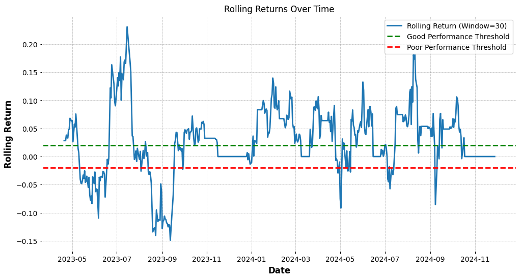
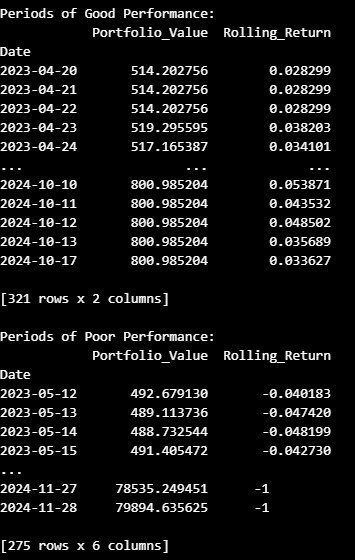
We analyze periods of good and poor performance and compare our strategy against a buy-and-hold approach.

# performance Periods analysis
test_data['Strategy_Return'] = test_data['Portfolio_Value'].pct_change()
test_data['Rolling_Return'] = test_data['Strategy_Return'].rolling(window=30).sum()

# periods of good performance
good_performance = test_data[test_data['Rolling_Return'] > 0.02]

# Periods of poor performance
poor_performance = test_data[test_data['Rolling_Return'] < -0.02]

# Plot Rolling Returns Over Time
plt.figure(figsize=(12, 6))
plt.plot(test_data.index, test_data['Rolling_Return'], label='Rolling Return (Window=30)')
plt.axhline(0.02, color='green', linestyle='--', label='Good Performance Threshold')
plt.axhline(-0.02, color='red', linestyle='--', label='Poor Performance Threshold')
plt.title('Rolling Returns Over Time')
plt.xlabel('Date')
plt.ylabel('Rolling Return')
plt.legend()
plt.show()

# Compare our strategy with Buy-and-Hold Strategy
test_data['Buy_and_Hold'] = initial_capital * (test_data['Actual_Close'] / test_data['Actual_Close'].iloc[0])

plt.figure(figsize=(12, 6))
plt.plot(test_data.index, test_data['Portfolio_Value'], label='Strategy Portfolio Value')
plt.plot(test_data.index, test_data['Buy_and_Hold'], label='Buy and Hold Portfolio Value')
plt.title('Portfolio Value Comparison')
plt.xlabel('Date')
plt.ylabel('Portfolio Value in USD')
plt.legend()
plt.show()

# Performance Periods
print("\nPeriods of Good Performance:")
if not good_performance.empty:
    print(good_performance[['Portfolio_Value', 'Rolling_Return']])
else:
    print("No periods of good performance found.")

print("\nPeriods of Poor Performance:")
if not poor_performance.empty:
    print(poor_performance[['Portfolio_Value', 'Rolling_Return']])
else:
    print("No periods of poor performance found.")