The Business Brief Executives Actually Trust

In a world of sensational headlines and shallow analysis, The Daily Upside stands apart. Founded by former bankers and seasoned journalists, it delivers crisp, actionable insights executives actually use to make smarter decisions.

From market-moving developments to deep dives on business trends, The Daily Upside gives leaders clarity on what matters — without the noise.

That’s why over 1 million readers, including C-suite executives and senior decision-makers, start their day with it.

No fluff. No spin. Just business clarity.

Subscribe free.

🚀 Your Investing Journey Just Got Better: Premium Subscriptions Are Here! 🚀

It’s been 4 months since we launched our premium subscription plans at GuruFinance Insights, and the results have been phenomenal! Now, we’re making it even better for you to take your investing game to the next level. Whether you’re just starting out or you’re a seasoned trader, our updated plans are designed to give you the tools, insights, and support you need to succeed.

Here’s what you’ll get as a premium member:

• Exclusive Trading Strategies: Unlock proven methods to maximize your returns.

• In-Depth Research Analysis: Stay ahead with insights from the latest market trends.

• Ad-Free Experience: Focus on what matters most—your investments.

• Monthly AMA Sessions: Get your questions answered by top industry experts.

• Coding Tutorials: Learn how to automate your trading strategies like a pro.

• Masterclasses & One-on-One Consultations: Elevate your skills with personalized guidance.

Our three tailored plans—Starter Investor, Pro Trader, and Elite Investor—are designed to fit your unique needs and goals. Whether you’re looking for foundational tools or advanced strategies, we’ve got you covered.

Don’t wait any longer to transform your investment strategy. The last 4 months have shown just how powerful these tools can be—now it’s your turn to experience the difference.

👉 Explore Premium Plans Now

I wanted to find out if a simple technical trading strategy called the Rate of Change (ROC), which looks at how much a price has changed over time, could help improve Bitcoin trading when used with some smart adjustments.

Instead of trying complicated methods, I focused on tuning this one indicator to see what it could do.

To find the best settings quickly, I used a method called Bayesian Optimization. It’s a way to test different options smartly without wasting time trying everything randomly.

📈 Algorithmic Trading Course

I’m launching a premium online course on algorithmic trading starting July 21. The price is $3000, and spots will be limited.

🔥 What to Expect:

• Build trading bots with Python

• Backtest strategies with real data

• Learn trend-following, mean-reversion, and more

• Live execution, portfolio risk management

• Bonus: machine learning & crypto trading modules

🎁 Free Bonus:

Everyone who enrolls will get a free e-book:
“100 Trading Strategies in Python” — full of ready-to-use code.

👉 Interested? Join the program now:
I want to get in

In this article, I’ll walk you through each step of the process:

1. Collecting and preparing the data

2. Splitting the data into training and testing sets

3. Defining the trading strategy

4. Optimizing the strategy’s parameters

5. Running backtests to evaluate performance

6. Comparing the results to a simple buy-and-hold approach with Bitcoin

Setup: Importing Libraries and Dependencies

First, I installed and imported all the libraries I needed, including:

• yfinance for stock data

• matplotlib for plotting

• ta library for technical analysis

• bayesian-optimization package for hyperparameter tuning.

%pip install yfinance bayesian-optimization matplotlib pandas ta tabulate --quiet

import yfinance as yf
import matplotlib.pyplot as plt
from ta.momentum import ROCIndicator
from bayes_opt import BayesianOptimization
from tabulate import tabulate
plt.style.use('dark_background')

Loading the Data

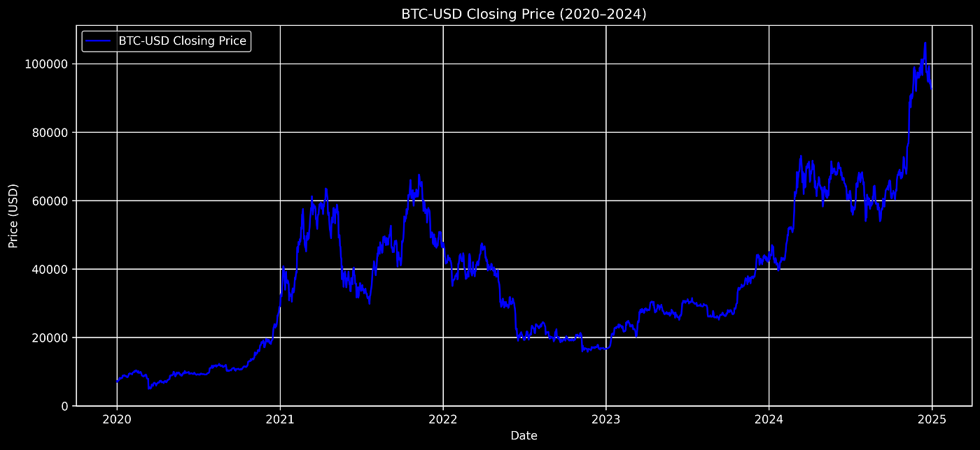
For this project, I chose Bitcoin (BTC-USD), given its volatility and popularity.

I downloaded daily closing prices from 2020 to the end of 2024.

# Load Bitcoin stock data
symbol = 'BTC-USD'
initial_cash = 1  # Initial cash for backtesting
data = yf.download(symbol, start='2020-01-01', end='2024-12-31')
data.columns = data.columns.get_level_values(0)
data = data[['Close']]
data.dropna(inplace=True)
data.head()

Visualizing Price Data

Before diving into strategy development, it’s important to understand the data visually.

Here’s the closing price chart over the selected period.

# Visualize the closing price of the stock
plt.figure(figsize=(14,6))
plt.plot(data.index, data['Close'], label=f'{symbol} Closing Price', color='blue')
plt.title(f'{symbol} Closing Price (2020–2024)')
plt.xlabel('Date')
plt.ylabel('Price (USD)')
plt.grid(True)
plt.legend()
plt.savefig('closing_price.png', dpi=300, bbox_inches='tight')
plt.show()

Train-Test Split

To ensure our strategy is evaluated fairly, I split the data into training (70%) and testing (30%) sets based on date.

# Train-test split (70% train, 30% test)
train_size = int(len(data) * 0.7)
train_data = data.iloc[:train_size].copy()
test_data = data.iloc[train_size:].copy()

print(f"Training from {train_data.index[0]} to {train_data.index[-1]}")
print(f"Testing from {test_data.index[0]} to {test_data.index[-1]}")

Output:

Training from 2020-01-01 to 2023-07-01
Testing from 2023-07-02 to 2024-12-30

Defining the Backtesting Function

This function takes the data and trading parameters, calculates the ROC indicator, and simulates buying and selling based on thresholds.

It tracks portfolio value over time and records trade signals.

def backtest_strategy(df, roc_window, buy_threshold, sell_threshold):
    df = df.copy()
    roc_window = int(roc_window)
    buy_threshold = float(buy_threshold)
    sell_threshold = float(sell_threshold)

    roc = ROCIndicator(close=df['Close'], window=roc_window)
    df['ROC'] = roc.roc()

    position = 0
    cash = initial_cash
    portfolio = []
    trades = 0
    buy_signals = []
    sell_signals = []

    for i in range(roc_window, len(df)):
        if df['ROC'].iloc[i] > buy_threshold and position == 0:
            position = cash / df['Close'].iloc[i]
            cash = 0
            buy_signals.append((df.index[i], df['Close'].iloc[i]))
            trades += 1
        elif df['ROC'].iloc[i] < sell_threshold and position > 0:
            cash = position * df['Close'].iloc[i]
            position = 0
            sell_signals.append((df.index[i], df['Close'].iloc[i]))
            trades += 1
        
        portfolio_value = cash + (position * df['Close'].iloc[i])
        portfolio.append(portfolio_value)

    final_value = cash + position * df['Close'].iloc[-1]
    return_percentage = (final_value - initial_cash) / initial_cash * 100

    return return_percentage, trades, buy_signals, sell_signals, portfolio

Objective Function for Bayesian Optimization

To tune the ROC window size and buy/sell thresholds, I defined an objective function that backtests the strategy on training data and returns the strategy’s return.

Bayesian Optimization will try to maximize this return.

def objective(roc_window, buy_threshold, sell_threshold):
    returns, _, _, _, _ = backtest_strategy(train_data, roc_window, buy_threshold, sell_threshold)
    return returns

Running Bayesian Optimization

I set bounds for each parameter and ran the optimizer for 20 iterations after 5 random initial points.

The output included the best parameters found.

pbounds = {
    'roc_window': (3, 30),
    'buy_threshold': (0.1, 10),
    'sell_threshold': (-10, -0.1)
}

optimizer = BayesianOptimization(
    f=objective,
    pbounds=pbounds,
    random_state=42,
    verbose=2
)

optimizer.maximize(init_points=5, n_iter=20)
best_params = optimizer.max['params']
best_params

Output:

{
   'roc_window': np.float64(27.943437909406587),
   'buy_threshold': np.float64(0.1),
   'sell_threshold': np.float64(-2.722477471437819)
}

Backtesting on Test Data Using Optimized Parameters

With the best parameters, I backtested the strategy on the test set to get final returns and trade counts.

best_roc = int(best_params['roc_window'])
best_buy = float(best_params['buy_threshold'])
best_sell = float(best_params['sell_threshold'])

returns, trades, buy_signals, sell_signals, portfolio = backtest_strategy(
    test_data, best_roc, best_buy, best_sell
)

print(f"Final Return on Test Set: {returns:.2f}%")
print(f"Number of Trades: {trades}")

Output:

Final Return on Test Set: 167.65%
Number of Trades: 24

Comparing Strategy vs Buy-and-Hold

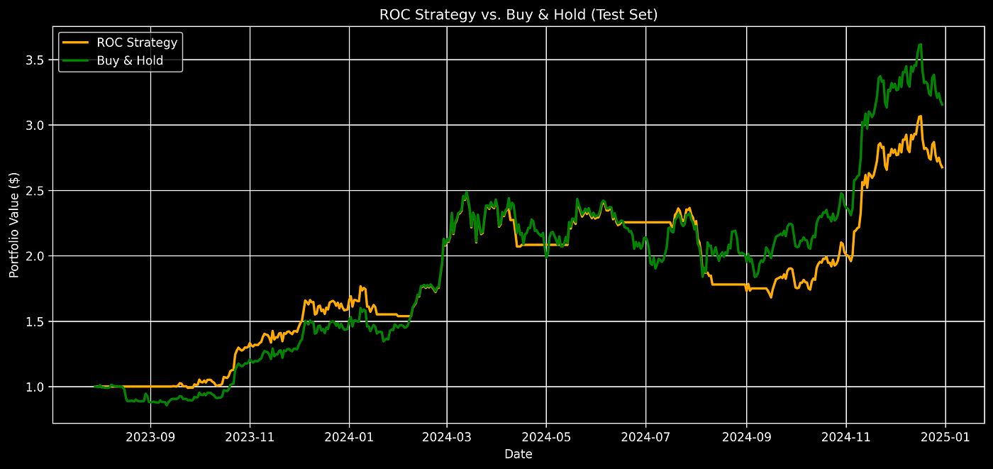
I then compared the portfolio value progression against a simple buy-and-hold strategy that keeps the asset for the entire test period.

# Visualize portfolio value vs. buy-and-hold on the test set
df = test_data.copy()
df = df.iloc[best_roc:].copy()  # Skip rows lost due to ROC calculation

# Strategy Portfolio Value
df['Strategy'] = portfolio

# Buy-and-hold simulation
initial_price = df['Close'].iloc[0]
df['BuyHold'] = (df['Close'] / initial_price) * initial_cash

# Plot both
plt.figure(figsize=(14,6))
plt.plot(df.index, df['Strategy'], label='ROC Strategy', color='orange')
plt.plot(df.index, df['BuyHold'], label='Buy & Hold', color='green')

plt.title('ROC Strategy vs. Buy & Hold (Test Set)')
plt.xlabel('Date')
plt.ylabel('Portfolio Value ($)')
plt.legend()
plt.grid(True)
plt.savefig('portfolio_comparison.png', dpi=300, bbox_inches='tight')
plt.show()

Visualizing Buy and Sell Signals

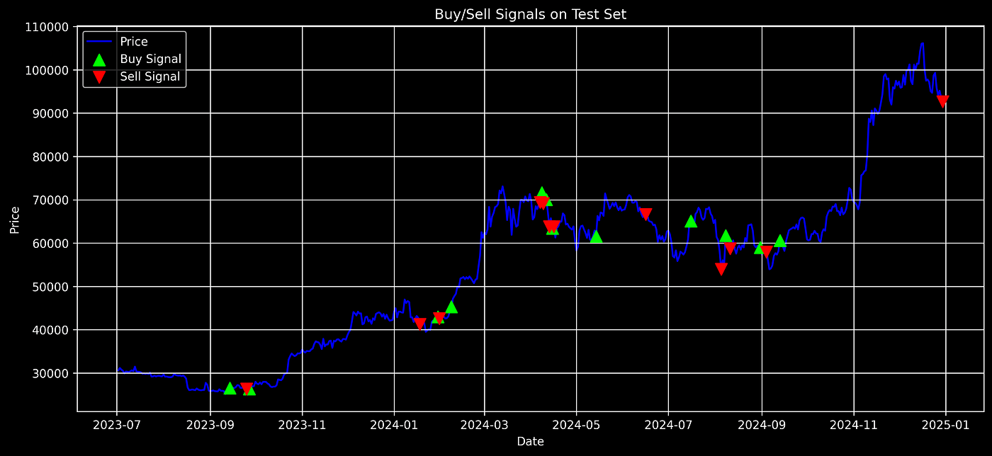
To get a clear picture of when the strategy was buying or selling, I plotted signals on top of the closing price.

# Plot buy/sell signals on test set
plt.figure(figsize=(14,6))

# Plot the closing price first
plt.plot(test_data.index, test_data['Close'], label='Price', color='blue', zorder=1)

# Plot buy signals
for buy in buy_signals:
    plt.scatter(buy[0], buy[1], marker='^', color='lime', s=100, label='Buy Signal', zorder=2)

# Plot sell signals
for sell in sell_signals:
    plt.scatter(sell[0], sell[1], marker='v', color='red', s=100, label='Sell Signal', zorder=2)

# Only show each label once
handles, labels = plt.gca().get_legend_handles_labels()
by_label = dict(zip(labels, handles))
plt.legend(by_label.values(), by_label.keys())

plt.title('Buy/Sell Signals on Test Set')
plt.xlabel('Date')
plt.ylabel('Price')
plt.grid(True)
plt.savefig('buy_sell_signals.png', dpi=300, bbox_inches='tight')
plt.show()

Final Performance Summary

Lastly, I summarized the performance metrics of the strategy alongside the buy-and-hold benchmark for easy comparison.

# Strategy evaluation
total_trades = len(buy_signals) + len(sell_signals)

if len(buy_signals) == len(sell_signals):
    successful_trades = sum(
        sell[1] > buy[1] for buy, sell in zip(buy_signals, sell_signals)
    )
    win_rate = f"{(successful_trades / len(sell_signals) * 100):.2f}%"
else:
    win_rate = 'Inconsistent buy/sell pairs'

test_df = test_data.copy().iloc[best_roc:].copy()  # align with portfolio calculation start
initial_price = test_df['Close'].iloc[0]
final_price = test_df['Close'].iloc[-1]

final_strategy_value = portfolio[-1]
final_bh_value = (final_price / initial_price) * initial_cash
bh_return_pct = (final_bh_value - initial_cash) / initial_cash * 100
strategy_return_pct = (final_strategy_value - initial_cash) / initial_cash * 100

summary = [
    ["Initial Cash", f"${initial_cash}", f"${initial_cash}"],
    ["Final Portfolio Value", f"${final_strategy_value:.2f}", f"${final_bh_value:.2f}"],
    ["Total Return (%)", f"{strategy_return_pct:.2f}%", f"{bh_return_pct:.2f}%"],
    ["Total Trades Executed", total_trades, "N/A"],
    ["Buy Trades", len(buy_signals), "N/A"],
    ["Sell Trades", len(sell_signals), "N/A"],
    ["Win Rate", win_rate, "N/A"]
]

print(tabulate(summary, headers=["Metric", "ROC Strategy", "Buy & Hold"], tablefmt="rounded_grid"))

Output:

╭───────────────────────┬────────────────┬──────────────╮
│ Metric                │ ROC Strategy   │ Buy & Hold   │
├───────────────────────┼────────────────┼──────────────┤
│ Initial Cash          │ $1             │ $1           │
├───────────────────────┼────────────────┼──────────────┤
│ Final Portfolio Value │ $2.68          │ $3.16        │
├───────────────────────┼────────────────┼──────────────┤
│ Total Return (%)      │ 167.65%        │ 215.58%      │
├───────────────────────┼────────────────┼──────────────┤
│ Total Trades Executed │ 24             │ N/A          │
├───────────────────────┼────────────────┼──────────────┤
│ Buy Trades            │ 12             │ N/A          │
├───────────────────────┼────────────────┼──────────────┤
│ Sell Trades           │ 12             │ N/A          │
├───────────────────────┼────────────────┼──────────────┤
│ Win Rate              │ 41.67%         │ N/A          │
╰───────────────────────┴────────────────┴──────────────╯

While the ROC strategy delivered a solid return of about 168%, it did not quite surpass the 216% return of simply holding Bitcoin over the same period.

The strategy executed 24 trades with a win rate of around 42%, showing that while it can capture gains, it also involves frequent trading and some losses.

This highlights the trade-off between active trading and a passive buy-and-hold approach, active management can offer opportunities but also carries risk and requires careful tuning.

For anyone exploring algorithmic trading, this exercise demonstrates how even a straightforward indicator combined with smart parameter optimization can produce meaningful results. It’s a practical starting point for developing and refining your own trading strategies.