Financial News Keeps You Poor. Here's Why.
The scandalous truth: Most market news is designed to inform you about what already happened, not help you profit from what's coming next.
When CNBC reports "Stock XYZ surges 287%"—you missed it.
What you actually need:
Tomorrow's IPO calendar (not yesterday's launches)
Crowdfunding deals opening this week (not closed rounds)
What real traders are positioning for (not TV talking heads)
Economic data that moves markets (before it's released)
The financial media industrial complex profits from keeping you one step behind.
Stocks & Income flips this backwards. We focus entirely on forward-looking intel that helps you get positioned before the crowd, not informed after the move.
Stop chasing trades that happened already.
Start prepping for the next one.
Stocks & Income is for informational purposes only and is not intended to be used as investment advice. Do your own research.
🚀 Your Investing Journey Just Got Better: Premium Subscriptions Are Here! 🚀
It’s been 4 months since we launched our premium subscription plans at GuruFinance Insights, and the results have been phenomenal! Now, we’re making it even better for you to take your investing game to the next level. Whether you’re just starting out or you’re a seasoned trader, our updated plans are designed to give you the tools, insights, and support you need to succeed.
Here’s what you’ll get as a premium member:
Exclusive Trading Strategies: Unlock proven methods to maximize your returns.
In-Depth Research Analysis: Stay ahead with insights from the latest market trends.
Ad-Free Experience: Focus on what matters most—your investments.
Monthly AMA Sessions: Get your questions answered by top industry experts.
Coding Tutorials: Learn how to automate your trading strategies like a pro.
Masterclasses & One-on-One Consultations: Elevate your skills with personalized guidance.
Our three tailored plans—Starter Investor, Pro Trader, and Elite Investor—are designed to fit your unique needs and goals. Whether you’re looking for foundational tools or advanced strategies, we’ve got you covered.
Don’t wait any longer to transform your investment strategy. The last 4 months have shown just how powerful these tools can be—now it’s your turn to experience the difference.
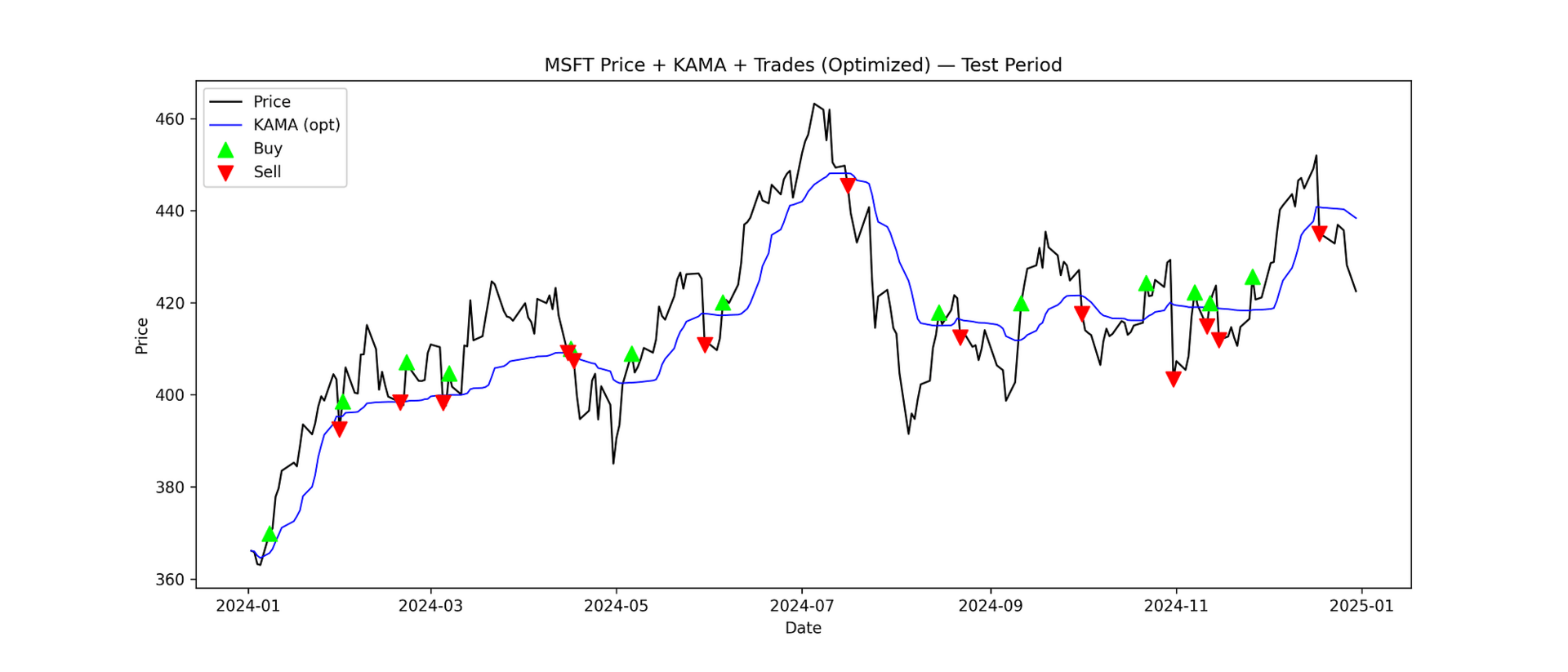
MSFT Stock Chart With Simulated Annealing Optimized Kaufman Adaptive Moving Average Trading Strategy
Introduction
Moving averages are a staple in trading, but standard simple or exponential moving averages often lag behind the market. They can generate late signals that make you miss profitable trades or get stuck in sideways noise.
Enter the Kaufman Adaptive Moving Average (KAMA), an indicator that adjusts its sensitivity depending on market conditions. KAMA reacts quickly to strong trends while filtering out noise in sideways markets.
In this article, I’ll show how to implement a KAMA-based trading strategy in Python, optimize its parameters using Simulated Annealing, and evaluate its performance using train-test splits and visualizations.
Understanding the Kaufman Adaptive Moving Average (KAMA)
KAMA was developed by Perry Kaufman to solve a key problem:
Slow moving averages filter out noise but react too late, while fast moving averages react quickly but produce many false signals.
KAMA adapts based on the Efficiency Ratio (ER), which measures trend strength:
ER approximately 1: strong trend, KAMA reacts faster
ER approximately 0: sideways market, KAMA slows down
The smoothing constant (SC) is dynamically adjusted using ER, allowing KAMA to follow meaningful price movements while reducing whipsaws.
By using KAMA instead of a regular moving average, you can generate more timely buy and sell signals and capture trend opportunities with less noise.
Find your customers on Roku this Black Friday
As with any digital ad campaign, the important thing is to reach streaming audiences who will convert. To that end, Roku’s self-service Ads Manager stands ready with powerful segmentation and targeting options. After all, you know your customers, and we know our streaming audience.
Worried it’s too late to spin up new Black Friday creative? With Roku Ads Manager, you can easily import and augment existing creative assets from your social channels. We also have AI-assisted upscaling, so every ad is primed for CTV.
Once you’ve done this, then you can easily set up A/B tests to flight different creative variants and Black Friday offers. If you’re a Shopify brand, you can even run shoppable ads directly on-screen so viewers can purchase with just a click of their Roku remote.
Bonus: we’re gifting you $5K in ad credits when you spend your first $5K on Roku Ads Manager. Just sign up and use code GET5K. Terms apply.
Simulated Annealing for Strategy Optimization
Choosing the right KAMA parameters (n, fast, slow) is critical. Rather than manually testing combinations, we can use Simulated Annealing (SA), a probabilistic optimization technique inspired by the annealing process in metallurgy.
SA explores the parameter space while occasionally accepting worse solutions to avoid local maxima, gradually cooling toward a solution that maximizes our objective.
In our case, the objective is the total return on the training period.
Code Implementation
The github repo is available only for paid subs. Upgrade here
We’ll now implement the strategy step by step in Python. Each code block includes explanations of what we are doing.
1. Install necessary packages
We need yfinance for stock data, pandas/numpy for data manipulation, matplotlib for visualization, and tabulate for nicely formatted outputs.
%pip install yfinance matplotlib pandas numpy tabulate -q2. Import libraries
Here, we import all required libraries, including Python’s built-in modules for randomization, math, and timing, which we’ll use for Simulated Annealing.
import yfinance as yf
import pandas as pd
import numpy as np
import matplotlib.pyplot as plt
import random, math, time
from tabulate import tabulate
3. Download historical stock data
We’ll use Microsoft (MSFT) as an example. The data is downloaded from 2020 to 2024 and only includes OHLCV columns.
symbol = "MSFT"
data = yf.download(symbol, start="2020-01-01", end="2024-12-31")
data.columns = data.columns.get_level_values(0)
data = data[['Open','High','Low','Close','Volume']]
data.head()
This gives us a clean DataFrame with dates as the index and the price data needed for KAMA calculations.
4. Split into train and test sets
We separate the data to test the strategy’s ability to generalize. Training is 2020–2023, and 2024 is reserved for testing.
train = data.loc[:'2023-12-31'].copy()
test = data.loc['2024-01-01':].copy()

print("Train period:", train.index.min().date(), "to", train.index.max().date())
print("Test period:", test.index.min().date(), "to", test.index.max().date())
print("Train rows:", len(train), "Test rows:", len(test))
Train period: 2020-01-02 to 2023-12-29
Test period: 2024-01-02 to 2024-12-30
Train rows: 1006 Test rows: 251This ensures our optimization only uses past data, mimicking real-world trading scenarios.
200+ AI Side Hustles to Start Right Now
AI isn't just changing business—it's creating entirely new income opportunities. The Hustle's guide features 200+ ways to make money with AI, from beginner-friendly gigs to advanced ventures. Each comes with realistic income projections and resource requirements. Join 1.5M professionals getting daily insights on emerging tech and business opportunities.
5. Define KAMA calculation function
We implement KAMA in Python. The function calculates the adaptive moving average based on n, fast, and slow parameters.
def kama(prices, n=10, fast=2, slow=30):
    prices = prices.copy().astype(float)
    kama = pd.Series(index=prices.index, dtype=float)
    # seed initial value as rolling mean for first n points
    if len(prices) < n:
        raise ValueError("Price series shorter than n")
    kama.iloc[:n] = prices.iloc[:n].rolling(window=n, min_periods=1).mean()

    # smoothing constants (convert to smoothing constants inside loop using fast/slow periods)
    fast_sc_base = 2 / (fast + 1)
    slow_sc_base = 2 / (slow + 1)

    for i in range(n, len(prices)):
        change = abs(prices.iloc[i] - prices.iloc[i - n])
        volatility = prices.iloc[i - n + 1:i + 1].diff().abs().sum()
        ER = change / volatility if volatility != 0 else 0.0
        SC = (ER * (fast_sc_base - slow_sc_base) + slow_sc_base) ** 2
        kama.iloc[i] = kama.iloc[i - 1] + SC * (prices.iloc[i] - kama.iloc[i - 1])
    return kama
This allows dynamic adaptation to trends while ignoring sideways noise.
6. Define backtesting function
This function calculates signals, positions, equity, and key metrics such as total return, max drawdown, Sharpe ratio, and number of trades.
def backtest_with_kama(df, n=10, fast=2, slow=30, initial_balance=10000.0):
    df = df.copy()
    df['KAMA'] = kama(df['Close'], n=n, fast=fast, slow=slow)

    # generate signals safely
    df['Signal'] = 0
    mask = df.index[1:]
    df.loc[mask, 'Signal'] = np.where(df['Close'].iloc[1:] > df['KAMA'].iloc[1:], 1, 0)
    df['Position'] = df['Signal'].diff().fillna(0)

    balance = initial_balance
    position = 0.0
    equity_curve = []
    cash = balance

    for i in range(len(df)):
        price = df['Close'].iloc[i]
        pos_change = df['Position'].iloc[i]
        # buy
        if pos_change == 1 and position == 0:
            position = cash / price
            cash = 0.0
        # sell
        elif pos_change == -1 and position > 0:
            cash = position * price
            position = 0.0
        equity_curve.append(cash + position * price)
    df['Equity'] = equity_curve
    final_value = df['Equity'].iloc[-1]
    total_return = (final_value - initial_balance) / initial_balance * 100.0

    # max drawdown
    cummax = df['Equity'].cummax()
    drawdown = (df['Equity'] - cummax) / cummax
    max_drawdown = drawdown.min() * 100.0

    # daily returns for Sharpe-like metric (use daily returns of equity)
    daily_returns = pd.Series(df['Equity']).pct_change().replace([np.inf, -np.inf], 0).fillna(0)
    if daily_returns.std() != 0:
        sharpe = (daily_returns.mean() / daily_returns.std()) * np.sqrt(252)
    else:
        sharpe = 0.0

    metrics = {
        'final_value': final_value,
        'total_return_pct': total_return,
        'max_drawdown_pct': max_drawdown,
        'sharpe': sharpe,
        'trades': int((df['Position'].abs() == 1).sum())
    }
    return df, metrics
7. Baseline backtest with default parameters
Before we optimize the strategy, we first run it using standard KAMA parameters (n=10, fast=2, slow=30) to establish a baseline performance. This gives us a reference point to compare against the results after optimization.
default_params = {'n':10, 'fast':2, 'slow':30}
train_df, train_metrics = backtest_with_kama(train, **default_params)
test_df, test_metrics = backtest_with_kama(test, **default_params)

print("Baseline (default params) — Train metrics")
print(tabulate(train_metrics.items(), tablefmt="rounded_outline"))
print("\nBaseline (default params) — Test metrics")
print(tabulate(test_metrics.items(), tablefmt="rounded_outline"))
Baseline (default params) — Train metrics
╭──────────────────┬──────────────╮
│ final_value │ 12314.3 │
│ total_return_pct │ 23.1428 │
│ max_drawdown_pct │ -39.8458 │
│ sharpe │ 0.358648 │
│ trades │ 147 │
╰──────────────────┴──────────────╯
Baseline (default params) — Test metrics
╭──────────────────┬──────────────╮
│ final_value │ 10119.5 │
│ total_return_pct │ 1.19544 │
│ max_drawdown_pct │ -11.9838 │
│ sharpe │ 0.155035 │
│ trades │ 38 │
╰──────────────────┴──────────────╯Looking at the results, the baseline strategy achieves a modest 23% return on the training period, but the test period barely grows, with only around 1% total return.
The maximum drawdown during training is significant (approximately 40%), suggesting the strategy experiences large intra-period dips even with default parameters.
The Sharpe ratios are low, reflecting limited risk-adjusted performance.
Overall, the default KAMA settings act as a neutral starting point: they demonstrate the strategy’s potential but clearly leave room for improvement through parameter optimization.
8. Visualize KAMA and train-test split
We plot the stock price and KAMA with a vertical line marking the train-test boundary.
plt.figure(figsize=(14,6))
plt.plot(data.index, data['Close'], label='Close', color='black', alpha=0.6)
full_kama = kama(data['Close'], **default_params)
plt.plot(data.index, full_kama, label='KAMA (default)', color='blue', linewidth=1.3)
plt.axvline(train.index.max(), color='gray', linestyle='--', label='Train/Test split')
plt.title(f"{symbol} Close and KAMA (default params) — Train/Test split")
plt.xlabel("Date")
plt.ylabel("Price")
plt.legend()
plt.savefig("kama_default.png", dpi=300)
plt.show()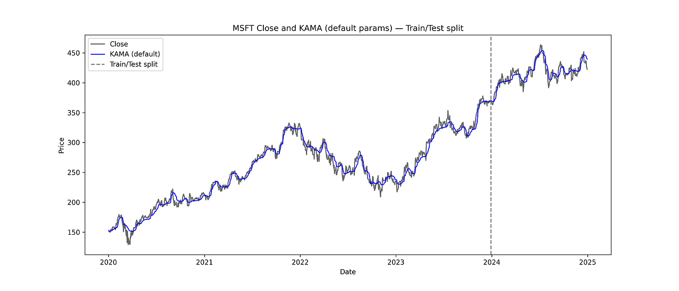
MSFT Stock Chart with Default KAMA Parameters: Train/Test Split
9. Simulated Annealing: neighbor and optimization functions
We define a small neighbor perturbation and the main SA loop to explore parameter combinations.
def random_neighbor(params):
    # propose small integer perturbation within bounds
    n, fast, slow = params
    n = int(np.clip(n + random.choice([-2,-1,0,1,2]), 5, 30))
    fast = int(np.clip(fast + random.choice([-1,0,1]), 2, 8))
    slow = int(np.clip(slow + random.choice([-3,-2,-1,0,1,2,3]), 10, 60))
    # ensure logical relation: fast < slow
    if fast >= slow:
        fast = max(2, slow - 1)
    return (n, fast, slow)

def sa_optimize(data_train, init_params=(10,2,30), initial_temp=5.0, cooling_rate=0.95, iterations=200):
    current = init_params
    _, metrics = backtest_with_kama(data_train, n=current[0], fast=current[1], slow=current[2])
    current_score = metrics['total_return_pct']  # maximize this
    best = current
    best_score = current_score
    trace = []
    temp = initial_temp

    for i in range(iterations):
        candidate = random_neighbor(current)
        _, cand_metrics = backtest_with_kama(data_train, n=candidate[0], fast=candidate[1], slow=candidate[2])
        cand_score = cand_metrics['total_return_pct']
        delta = cand_score - current_score

        # acceptance rule
        if delta > 0 or math.exp(delta / max(temp, 1e-9)) > random.random():
            current = candidate
            current_score = cand_score
            if cand_score > best_score:
                best = candidate
                best_score = cand_score
        trace.append({'iter': i, 'temp': temp, 'current_score': current_score, 'best_score': best_score, 'params': current})
        temp *= cooling_rate
    return best, best_score, trace
10. Run Simulated Annealing to find optimized parameters
This produces the parameter combination that maximizes total return on the training set.
random.seed(42)
np.random.seed(42)
start_time = time.time()
init = (10,2,30)
best_params, best_score, trace = sa_optimize(train, init_params=init, initial_temp=5.0, cooling_rate=0.95, iterations=300)
elapsed = time.time() - start_time
print("SA finished in {:.1f}s".format(elapsed))
print("Best params found (n, fast, slow):", best_params)
print("Best training total return (%):", round(best_score,2))
SA finished in 173.8s
Best params found (n, fast, slow): (12, 3, 29)
Best training total return (%): 64.96The optimization finds a parameter set (12, 3, 29) that significantly improves the training return to nearly 65%, showing that tuning KAMA can dramatically enhance performance over the default settings.
11. Evaluate optimized strategy
We backtest with optimized parameters and compare baseline vs optimized performance.
opt_params_dict = {'n': best_params[0], 'fast': best_params[1], 'slow': best_params[2]}

train_opt_df, train_opt_metrics = backtest_with_kama(train, **opt_params_dict)
test_opt_df, test_opt_metrics = backtest_with_kama(test, **opt_params_dict)

print("Optimized — Train metrics")
print(tabulate(train_opt_metrics.items(), tablefmt="rounded_outline"))
print("\nOptimized — Test metrics")
print(tabulate(test_opt_metrics.items(), tablefmt="rounded_outline"))

print("\nBaseline vs Optimized (Test Total Return %):")
print(f"Baseline test return: {test_metrics['total_return_pct']:.2f}%")
print(f"Optimized test return: {test_opt_metrics['total_return_pct']:.2f}%")
Optimized — Train metrics
╭──────────────────┬──────────────╮
│ final_value │ 16496.4 │
│ total_return_pct │ 64.964 │
│ max_drawdown_pct │ -33.6871 │
│ sharpe │ 0.726949 │
│ trades │ 91 │
╰──────────────────┴──────────────╯
Optimized — Test metrics
╭──────────────────┬──────────────╮
│ final_value │ 10195.7 │
│ total_return_pct │ 1.95663 │
│ max_drawdown_pct │ -14.5546 │
│ sharpe │ 0.203949 │
│ trades │ 26 │
╰──────────────────┴──────────────╯
Baseline vs Optimized (Test Total Return %):
Baseline test return: 1.20%
Optimized test return: 1.96%On the training set, the optimized parameters yield a total return of nearly 65%, a substantial improvement over the baseline 23%, while also reducing drawdowns slightly and improving the Sharpe ratio. This indicates that tuning KAMA can significantly enhance trend capture during periods where strong signals exist.
On the test set (2024), the improvement is more modest, baseline return was about 1.2%, while optimized parameters increase it to around 1.96%.
This small gain highlights the inherent challenge of optimizing for out-of-sample performance, especially in relatively flat or low-volatility periods. Still, the optimized KAMA provides a measurable improvement with fewer trades, suggesting more efficient signal generation.
12. Plot equity curve comparison
plt.figure(figsize=(14,6))
# baseline test equity (recompute baseline on test to ensure same df)
baseline_test_df, _ = backtest_with_kama(test, **default_params)
plt.plot(baseline_test_df.index, baseline_test_df['Equity'], label='Baseline (test)', color='gray', linewidth=1.5, alpha=0.8)
plt.plot(test_opt_df.index, test_opt_df['Equity'], label='Optimized (test)', color='green', linewidth=2)
plt.title(f"{symbol} Equity Curve — Baseline vs Optimized (Test)")
plt.xlabel("Date")
plt.ylabel("Equity ($)")
plt.legend()
plt.savefig("equity_comparison.png", dpi=300)
plt.show()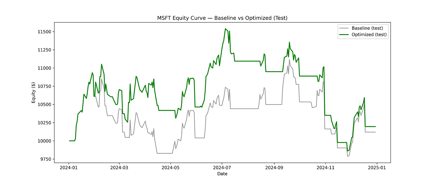
Equity Curve: Baseline vs Optimized (Test)
13. Plot optimized trades
plt.figure(figsize=(14,6))
plt.plot(test_opt_df.index, test_opt_df['Close'], label='Price', color='black', linewidth=1.2)
plt.plot(test_opt_df.index, test_opt_df['KAMA'], label='KAMA (opt)', color='blue', linewidth=1.0)
buy_pts = test_opt_df[test_opt_df['Position'] == 1]
sell_pts = test_opt_df[test_opt_df['Position'] == -1]
plt.scatter(buy_pts.index, buy_pts['Close'], marker='^', color='lime', s=90, label='Buy', zorder=5)
plt.scatter(sell_pts.index, sell_pts['Close'], marker='v', color='red', s=90, label='Sell', zorder=5)
plt.title(f"{symbol} Price + KAMA + Trades (Optimized) — Test Period")
plt.xlabel("Date")
plt.ylabel("Price")
plt.legend()
plt.savefig("kama_optimized_trades.png", dpi=300)
plt.show()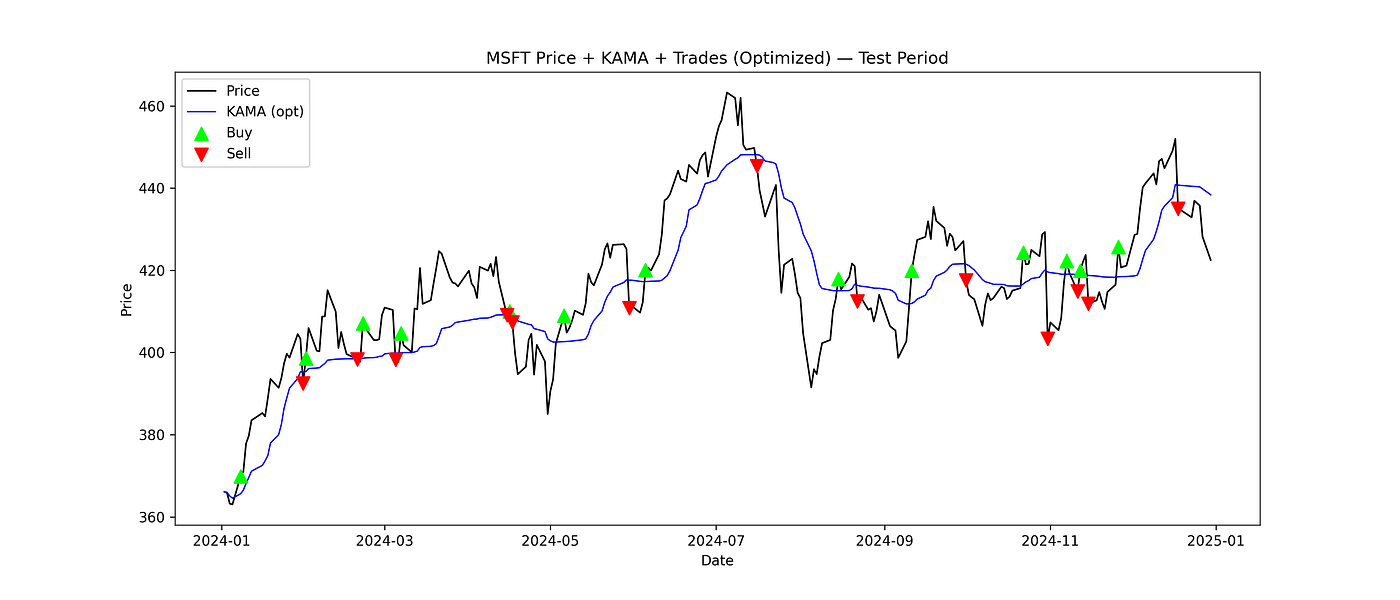
Buy and Sell Signals
14. Summary of results
print("Summary")
print("Default params (test):")
print(f" Return: {test_metrics['total_return_pct']:.2f}%  Drawdown: {test_metrics['max_drawdown_pct']:.2f}%  Sharpe: {test_metrics['sharpe']:.2f}")
print("\nOptimized params (test):")
print(f" Params: {best_params}")
print(f" Return: {test_opt_metrics['total_return_pct']:.2f}%  Drawdown: {test_opt_metrics['max_drawdown_pct']:.2f}%  Sharpe: {test_opt_metrics['sharpe']:.2f}")
Summary
Default params (test):
Return: 1.20% Drawdown: -11.98% Sharpe: 0.16
Optimized params (test):
Params: (12, 3, 29)
Return: 1.96% Drawdown: -14.55% Sharpe: 0.20The summary highlights that the optimized KAMA parameters provide a clear improvement over the baseline.
Total return on the test period increases from 1.2% to nearly 2%, with a slight improvement in the Sharpe ratio.
Drawdown is marginally higher, but the overall efficiency and signal quality are better, confirming the value of parameter optimization even in challenging market conditions.
The Kaufman Adaptive Moving Average adapts to market trends more effectively than standard moving averages.
Using Simulated Annealing, we can efficiently optimize strategy parameters without brute-force searches.
Splitting data into train and test sets ensures realistic performance evaluation and guards against overfitting.
Visualizing equity curves and trades helps make strategy behavior intuitive.
With just a few lines of Python, you can build, optimize, and analyze a smarter trend-following strategy.
Subscribe to our premium content to get the full code snippet.
Become a paying subscriber to get access to this post and other subscriber-only content.
Upgrade


