
In partnership with

Could you afford $3,500 to remove a chew toy?

From $3,500 to remove a chew toy, to $7,000 for a hip replacement, keeping your pets healthy is getting more and more expensive. Fortunately, pet insurance can help offset these rising costs. Pet insurance can cover eligible accidents and illnesses with up to 90% reimbursement. Get your buddy covered today with plans starting at just $10 a month.
🚀 Your Investing Journey Just Got Better: Premium Subscriptions Are Here! 🚀
It’s been 4 months since we launched our premium subscription plans at GuruFinance Insights, and the results have been phenomenal! Now, we’re making it even better for you to take your investing game to the next level. Whether you’re just starting out or you’re a seasoned trader, our updated plans are designed to give you the tools, insights, and support you need to succeed.
Here’s what you’ll get as a premium member:
Exclusive Trading Strategies: Unlock proven methods to maximize your returns.
In-Depth Research Analysis: Stay ahead with insights from the latest market trends.
Ad-Free Experience: Focus on what matters most—your investments.
Monthly AMA Sessions: Get your questions answered by top industry experts.
Coding Tutorials: Learn how to automate your trading strategies like a pro.
Masterclasses & One-on-One Consultations: Elevate your skills with personalized guidance.
Our three tailored plans—Starter Investor, Pro Trader, and Elite Investor—are designed to fit your unique needs and goals. Whether you’re looking for foundational tools or advanced strategies, we’ve got you covered.
Don’t wait any longer to transform your investment strategy. The last 4 months have shown just how powerful these tools can be—now it’s your turn to experience the difference.

Correlation Between Bitcoin Price Features
In this article, we will explore how to collect and process historical Bitcoin price data to create meaningful features for machine learning models.
We will use Python libraries to download the data, calculate key indicators, and visualize them.
These features can later be used for forecasting or predictive modeling.
Stay In The Business Know with 1440

Are you looking for easy breakdowns and knowledge deep dives on the latest key concepts to help you understand business and finance topics? Finance news doesn’t have to be confusing. 1440’s weekly newsletter explains markets, policy, and investing in plain English—complete with charts, context, and links to learn more.
Introduction
Bitcoin is one of the most widely traded cryptocurrencies, and its price has shown significant volatility since its inception.
To predict Bitcoin’s price movements, it is essential to build a dataset enriched with technical features derived from the raw price data.
This article walks through the process of downloading Bitcoin price data from Yahoo Finance using the yfinance API and generating several commonly used features such as:
Moving Averages
Bollinger Bands
Relative Strength Index (RSI)
Volatility
Python Implementation
All the code in this guide is made available for free. Check out the full link at the end of this article.
Before starting, we install and import all the necessary Python libraries:
%pip install yfinance matplotlib seaborn pandas numpy scikit-learnWe import the libraries and prepare the environment:
import yfinance as yf
import matplotlib.pyplot as plt
import pandas as pd
import numpy as np
import seaborn as sns
import os

plt.style.use("dark_background")

# Create directory to save plots
os.makedirs("figures", exist_ok=True)yfinanceis used to download historical price data.matplotlibandseabornare used for visualizations,while
pandasandnumpyhandle data processing.
Downloading and Inspecting Bitcoin Data
We download all available historical Bitcoin prices starting from 2014 and retain the key columns: Open, Close, Volume, Low, and High.
btc = yf.download("BTC-USD", start="2014-01-01")
btc.columns = btc.columns.get_level_values(0)
btc = btc[['Open', 'Close', 'Volume', 'Low', 'High']]

# Display first few rows
btc.head()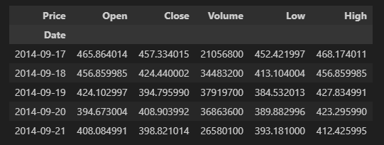
Top 5 Rows of Bitcoin Data
To understand the dataset, we check its date range, null values, data types, and basic statistics:
Range
print("Data range:", btc.index.min(), "to", btc.index.max())Data range: 2014-09-17 00:00:00 to 2025-05-25 00:00:00Missing Values
btc.isnull().sum()Price
Open 0
Close 0
Volume 0
Low 0
High 0
dtype: int64Data Types
btc.dtypesPrice
Open float64
Close float64
Volume int64
Low float64
High float64
dtype: objectStatistics
btc.describe()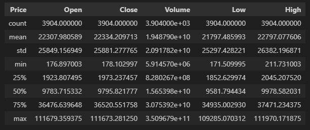
Bitcoin Dataset Statistics Summary
This step ensures the data is clean and covers the desired period.
Calculating Daily Returns
Daily return is the percentage change in the closing price compared to the previous day. It is a fundamental measure of asset performance and volatility.
btc["daily_return"] = btc["Close"].pct_change()
btc.dropna(inplace=True)
Next, we visualize the daily returns over time:
plt.figure(figsize=(14, 5))
plt.plot(btc.index, btc["daily_return"], label="Daily Return", color="purple")
plt.axhline(0, color="black", linestyle="--", linewidth=1)
plt.title("Bitcoin Daily Returns")
plt.xlabel("Date")
plt.ylabel("Daily Return")
plt.tight_layout()
plt.savefig("figures/btc_daily_returns.png")
plt.show()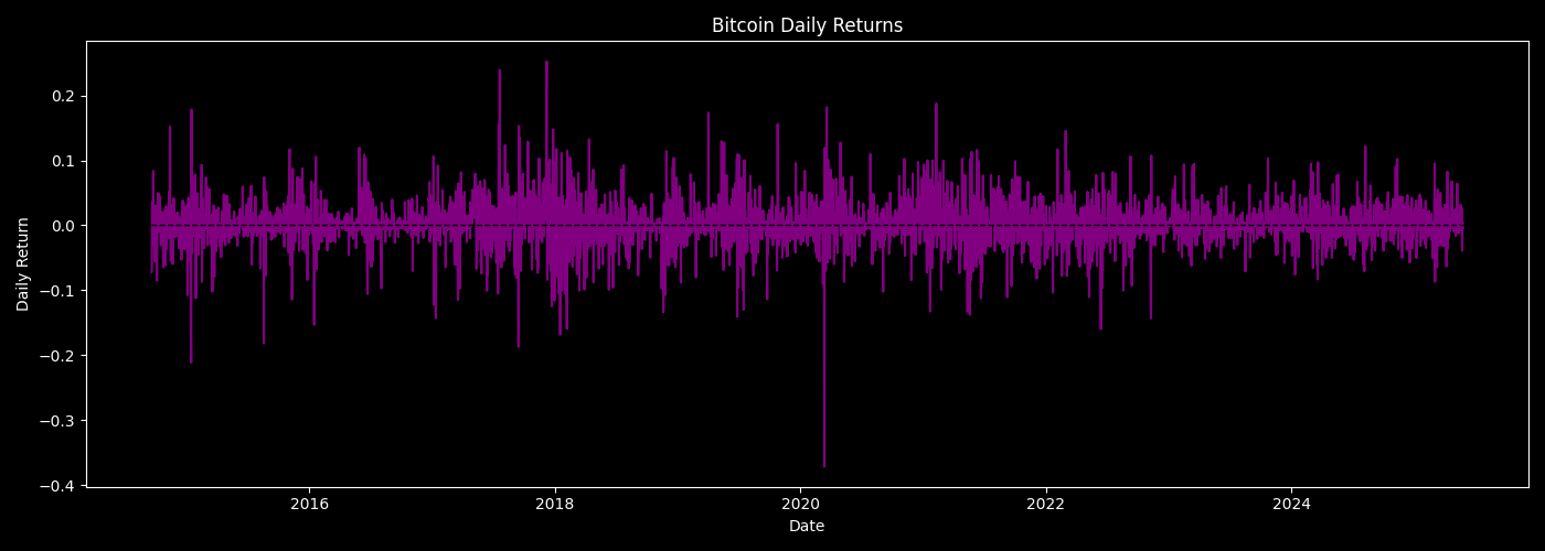
Bitcoin Daily Returns Plot
The plot reveals the highly volatile nature of Bitcoin price changes.
Adding Moving Averages
Moving averages smooth out price data to reveal trends over time. We calculate 7-day, 30-day, and 90-day moving averages:
btc["ma_7"] = btc["Close"].rolling(window=7).mean()
btc["ma_30"] = btc["Close"].rolling(window=30).mean()
btc["ma_90"] = btc["Close"].rolling(window=90).mean()
btc.dropna(inplace=True)
Visualizing the closing price with these moving averages provides insight into trend direction and strength:
plt.figure(figsize=(14, 6))
plt.plot(btc.index, btc["Close"], label="Closing Price", color="blue")
plt.plot(btc.index, btc["ma_30"], label="30-day MA", color="orange")
plt.plot(btc.index, btc["ma_90"], label="90-day MA", color="green")
plt.title("Bitcoin Closing Price with Moving Averages")
plt.xlabel("Date")
plt.ylabel("Price (USD)")
plt.legend()
plt.tight_layout()
plt.savefig("figures/btc_price_ma.png")
plt.show()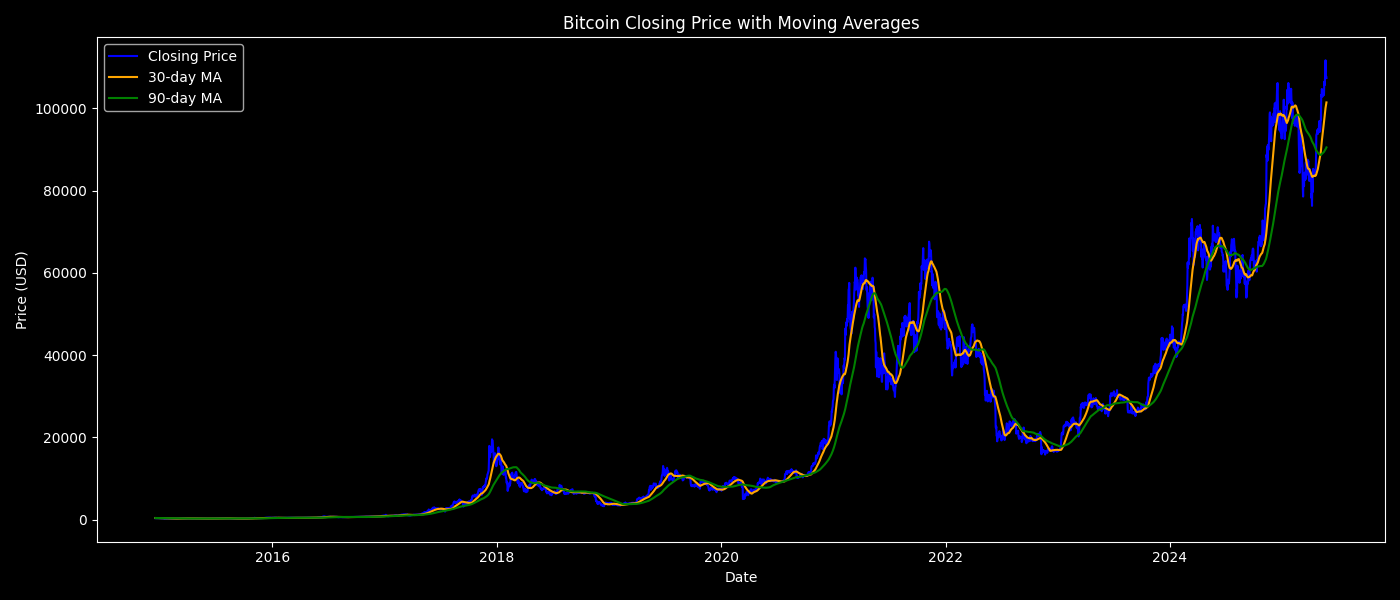
Bitcoin Closing Price with Moving Averages Chart
Calculating Bollinger Bands
Bollinger Bands use a moving average and standard deviation to indicate price volatility and potential overbought or oversold conditions.
We calculate 20-day moving average and standard deviation, then define upper and lower bands:
btc["ma_20"] = btc["Close"].rolling(window=20).mean()
btc["std_20"] = btc["Close"].rolling(window=20).std()
btc["upper_band"] = btc["ma_20"] + 2 * btc["std_20"]
btc["lower_band"] = btc["ma_20"] - 2 * btc["std_20"]
btc.dropna(inplace=True)
Plotting these bands alongside the closing price helps visualize periods of high and low volatility:
plt.figure(figsize=(14, 6))
plt.plot(btc.index, btc["Close"], label="Closing Price", color="blue")
plt.plot(btc.index, btc["upper_band"], label="Upper Band", linestyle="--", color="red")
plt.plot(btc.index, btc["lower_band"], label="Lower Band", linestyle="--", color="green")
plt.title("Bollinger Bands")
plt.xlabel("Date")
plt.ylabel("Price")
plt.legend()
plt.tight_layout()
plt.savefig("figures/btc_bollinger_bands.png")
plt.show()
Closing Price and Bollinger Bands Chart
Computing Relative Strength Index (RSI)
RSI measures momentum and indicates overbought or oversold conditions. It ranges from 0 to 100 and is calculated based on average gains and losses over a 14-day period.
delta = btc["Close"].diff()
gain = np.where(delta > 0, delta, 0)
loss = np.where(delta < 0, -delta, 0)

avg_gain = pd.Series(gain, index=btc.index).rolling(window=14).mean()
avg_loss = pd.Series(loss, index=btc.index).rolling(window=14).mean()

rs = avg_gain / avg_loss
btc["rsi_14"] = 100 - (100 / (1 + rs))
The RSI is visualized along with overbought (70) and oversold (30) thresholds:
plt.figure(figsize=(14, 5))
plt.plot(btc.index, btc["rsi_14"], label="RSI (14-day)", color="cyan")
plt.axhline(70, color="red", linestyle="--", linewidth=1, label="Overbought (70)")
plt.axhline(30, color="green", linestyle="--", linewidth=1, label="Oversold (30)")
plt.title("Bitcoin RSI (14-day)")
plt.xlabel("Date")
plt.ylabel("RSI")
plt.legend(loc="upper left")
plt.tight_layout()
plt.savefig("figures/btc_rsi_14.png")
plt.show()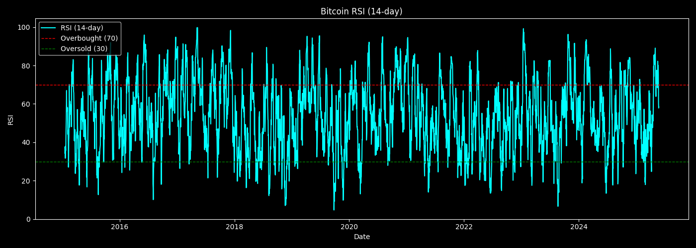
Bitcoin 14 day RSI
Calculating Rolling Volatility
Volatility reflects the risk or variability of returns. We compute 30-day rolling standard deviation of daily returns to measure volatility over time:
btc["volatility_30"] = btc["daily_return"].rolling(window=30).std()
btc.dropna(inplace=True)
Plotting the rolling volatility highlights periods when Bitcoin experienced large price fluctuations:
plt.figure(figsize=(14, 5))
plt.plot(btc.index, btc["volatility_30"], label="30-Day Rolling Volatility", color="crimson")
plt.title("Bitcoin Volatility (30-day Rolling Std Dev)")
plt.xlabel("Date")
plt.ylabel("Volatility")
plt.tight_layout()
plt.savefig("figures/btc_volatility.png")
plt.show()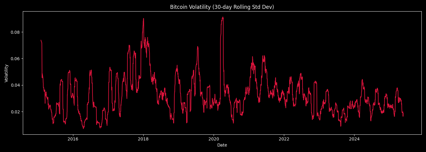
Bitcoin Volatility (30-day Rolling Std Dev) Chart
Saving and Inspecting Final Feature Set
All engineered features are saved for later modeling:
btc.to_csv("btc_features.csv", index=False)We can view the last few rows of all features:
features = btc.columns.tolist()
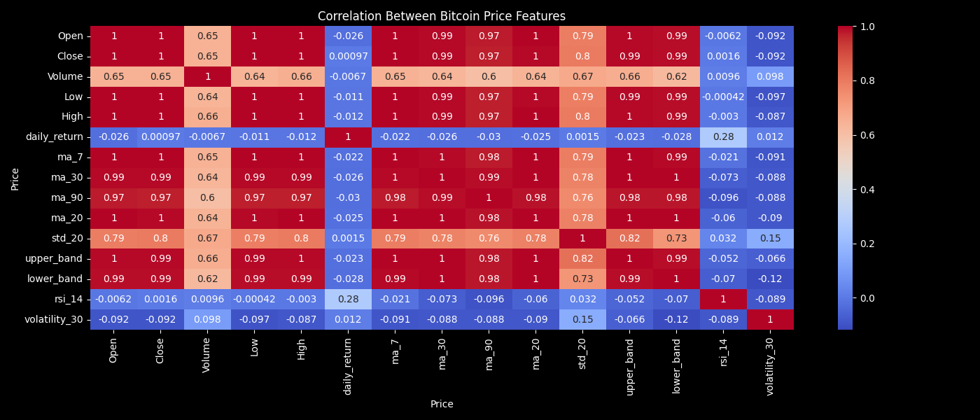
btc[features].tail()Finally, a correlation heatmap visualizes the relationships between features:
plt.figure(figsize=(14, 6))
sns.heatmap(btc[features].corr(), annot=True, cmap="coolwarm")
plt.title("Correlation Between Bitcoin Price Features")
plt.tight_layout()
plt.savefig("figures/btc_correlation_heatmap.png")
plt.show()
Bitcoin Features Correlation Heatmap
Conclusion
This article demonstrated how to download Bitcoin historical price data and construct important technical features.
These features capture trend, momentum, volatility, and price behavior, and serve as a foundation for predictive machine learning models.