
In partnership with

What Top Execs Read Before the Market Opens

The Daily Upside was founded by investment professionals to arm decision-makers with market intelligence that goes deeper than headlines. No filler. Just concise, trusted insights on business trends, deal flow, and economic shifts—read by leaders at top firms across finance, tech, and beyond.
🚀 Your Investing Journey Just Got Better: Premium Subscriptions Are Here! 🚀
It’s been 4 months since we launched our premium subscription plans at GuruFinance Insights, and the results have been phenomenal! Now, we’re making it even better for you to take your investing game to the next level. Whether you’re just starting out or you’re a seasoned trader, our updated plans are designed to give you the tools, insights, and support you need to succeed.
Here’s what you’ll get as a premium member:
Exclusive Trading Strategies: Unlock proven methods to maximize your returns.
In-Depth Research Analysis: Stay ahead with insights from the latest market trends.
Ad-Free Experience: Focus on what matters most—your investments.
Monthly AMA Sessions: Get your questions answered by top industry experts.
Coding Tutorials: Learn how to automate your trading strategies like a pro.
Masterclasses & One-on-One Consultations: Elevate your skills with personalized guidance.
Our three tailored plans—Starter Investor, Pro Trader, and Elite Investor—are designed to fit your unique needs and goals. Whether you’re looking for foundational tools or advanced strategies, we’ve got you covered.
Don’t wait any longer to transform your investment strategy. The last 4 months have shown just how powerful these tools can be—now it’s your turn to experience the difference.


Predicted Market Direction vs Close Price
Stock price predictions are a key part of trading, and machine learning offers powerful tools to make these predictions more accurate.
In this article, we’ll show how to train a Random Forest classifier to predict Tesla’s stock direction using historical data.
We’ll cover the steps involved, explain the features, and discuss why Random Forest is a strong choice for this kind of task.
Stock Price Prediction
Stock price prediction is an essential aspect of algorithmic trading and investment strategies. By predicting whether a stock’s price will go up (bullish) or down (bearish), traders can make informed decisions.
For this exercise, we will focus on Tesla (TSLA), one of the most volatile and widely followed stocks in the market.
We will use historical data from Yahoo Finance to train a Random Forest classifier, a robust and versatile model that can handle complex, non-linear relationships in data.
Setting Up the Environment
You can find the complete code for this project on my GitHub repository here.
Before we dive into the data, we need to install the necessary libraries using the following code:
%pip install yfinance matplotlib scikit-learn seabornThese libraries include:
yfinance for downloading stock data.
matplotlib and seaborn for visualizing the data.
scikit-learn for implementing the Random Forest classifier and other machine learning tools.
Downloading and Preprocessing Data
Next, we will use yfinance to download Tesla’s historical stock data. We will retrieve the data from 01 January 2010, to 31 December 2023, with a weekly interval.
We start by importing all the necessary libraries we are going to need in this project:
import yfinance as yf
import matplotlib.pyplot as plt
import seaborn as sns
from sklearn.ensemble import RandomForestClassifier
from sklearn.model_selection import train_test_split
from sklearn.metrics import classification_report, confusion_matrix

plt.style.use('dark_background')
data = yf.download("TSLA", start="2010-01-01", end="2023-12-31", auto_adjust=True, interval="1wk")
data.head()After downloading the data, we clean it by keeping only the relevant columns (Open, Close, Volume, Low, High), and we ensure the data is in a clean format by setting the columns properly.
data.columns = data.columns.get_level_values(0)
data = data[['Open', 'Close', 'Volume', 'Low', 'High']]
Visualizing the Data
Visualizing the data is an important step in understanding its behavior. We will plot the stock’s Open, Close, Low, and High prices over time to get a sense of the price fluctuations.
Plotting Function
# Function to plot individual features
def plot_feature(data, feature, color, title, ylabel):
    plt.figure(figsize=(14, 6))
    plt.plot(data.index, data[feature], label=feature, color=color)
    plt.title(title)
    plt.xlabel('Date')
    plt.ylabel(ylabel)
    plt.legend()
    plt.grid(True)
    plt.savefig(f"{feature}.png")
    plt.show()
Open
plot_feature(data, 'Open', 'green', 'Open Price Over Time', 'Open Price (USD)')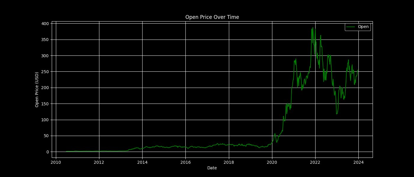
Open Price Over Time
Close
plot_feature(data, 'Close', 'blue', 'Close Price Over Time', 'Close Price (USD)')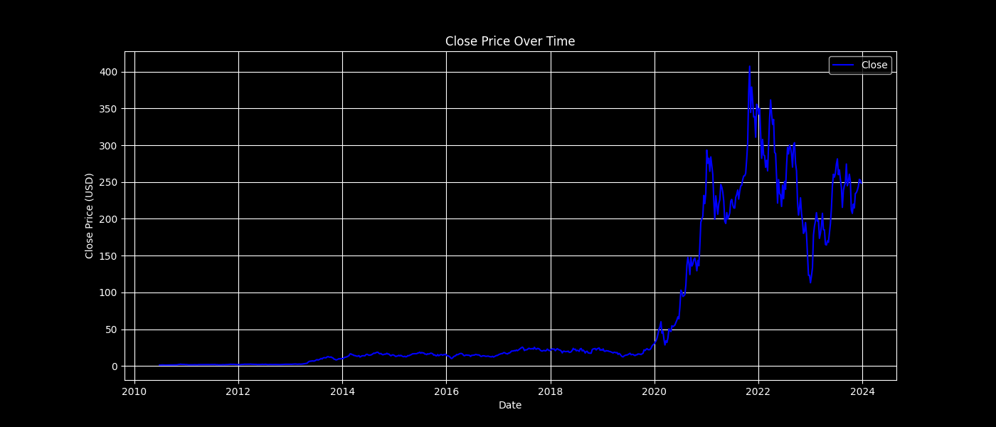
Close Price Over Time
Volume
plot_feature(data, 'Volume', 'orange', 'Volume Over Time', 'Volume')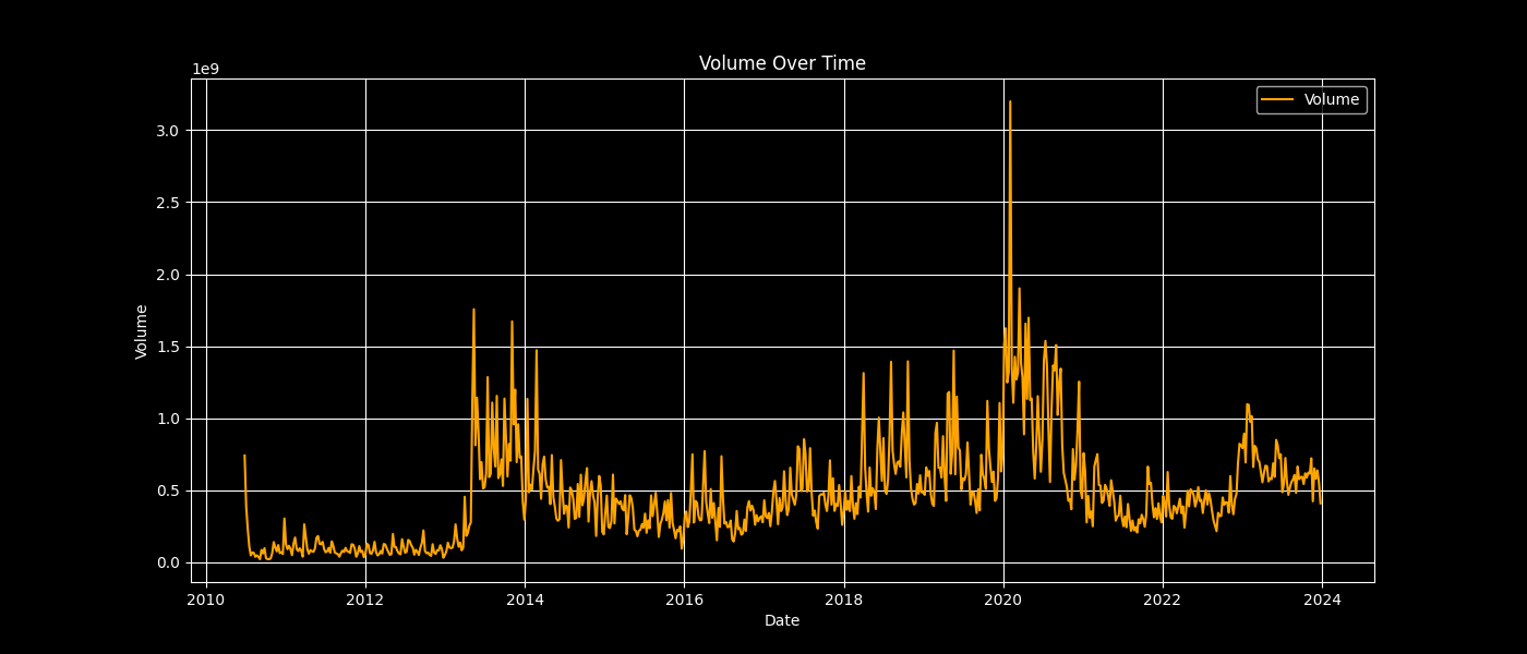
Volume Over Time
Low
plot_feature(data, 'Low', 'red', 'Low Price Over Time', 'Low Price (USD)')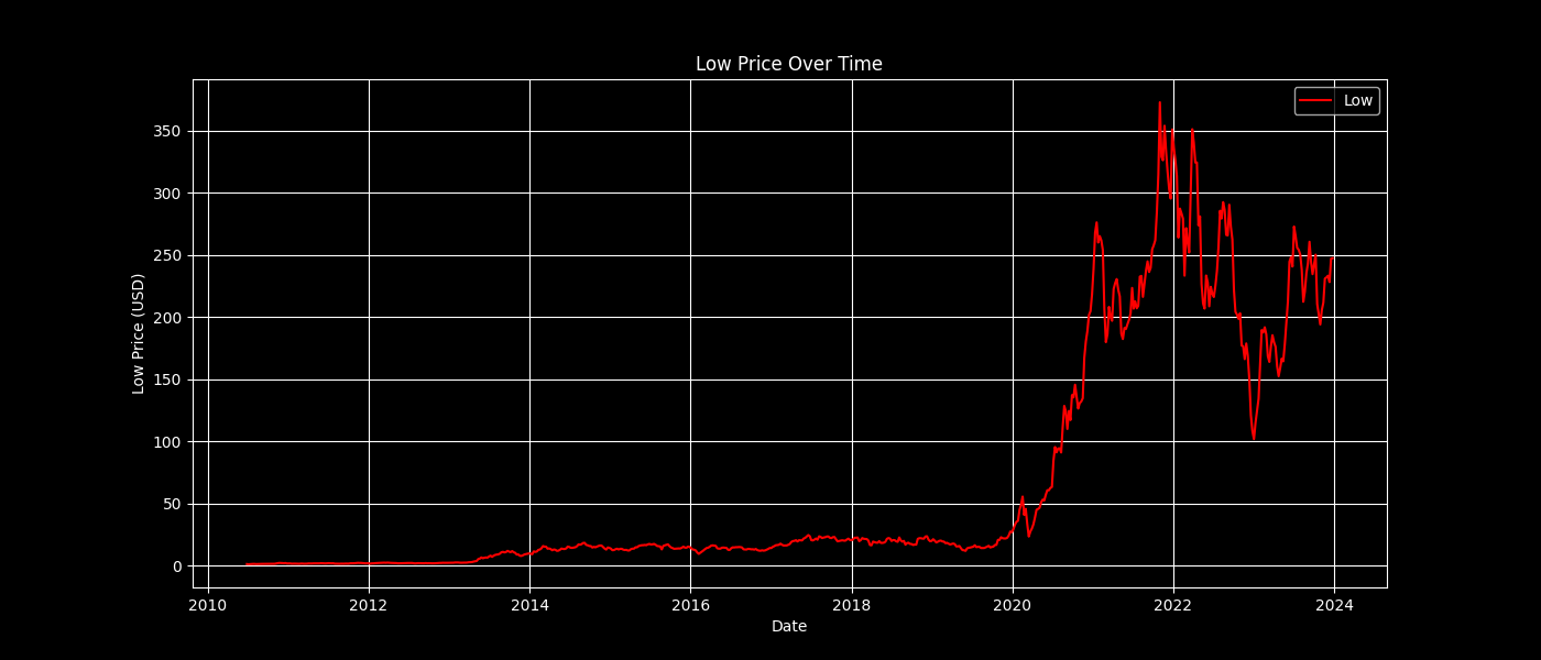
Low Price Over Time
High
plot_feature(data, 'High', 'purple', 'High Price Over Time', 'High Price (USD)')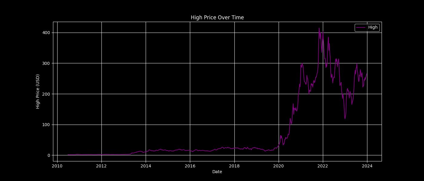
High Price Over Time
This allows us to observe the historical trends and volatility of Tesla’s stock.
Feature Engineering: Creating the Target Variable
To predict the stock’s direction (up or down), we need to define a target variable.
We will create a new column, “Direction”, which is
1 if the next day’s closing price is higher than the current day’s closing price, and
0 if it’s lower. This will allow us to classify whether the stock is going up or down.
data["Direction"] = (data["Close"].shift(-1) > data["Close"]).astype(int)
data.dropna(inplace=True)
Defining Features and Splitting the Data
For feature engineering, we will use the stock’s Open, Close, Low, High, and Volume data as features. These features are commonly used in technical analysis and provide a basis for predicting price movements.
X = data[['Open', 'Close', 'Volume', 'Low', 'High']]
y = data["Direction"]
We split the data into training and testing sets, with 80% of the data used for training and 20% for testing. We set shuffle=False to maintain the chronological order of the data.
X_train, X_test, y_train, y_test = train_test_split(X, y, test_size=0.2, random_state=42, shuffle=False)Training the Random Forest Classifier
Now, we can train the Random Forest classifier. This ensemble method builds multiple decision trees and merges them to get a more accurate and stable prediction.
We choose class_weight='balanced' to handle any class imbalance.
model = RandomForestClassifier(n_estimators=100, random_state=42, class_weight='balanced')
model.fit(X_train, y_train)
Evaluating the Model
After training the model, we evaluate its performance by predicting the stock’s direction on the test set.
We will also display the classification report and confusion matrix to assess how well the model distinguishes between upward and downward price movements.
Classification Report
y_pred = model.predict(X_test)
print(classification_report(y_test, y_pred))
precision recall f1-score support
0 0.52 0.55 0.54 67
1 0.57 0.54 0.56 74
accuracy 0.55 141
macro avg 0.55 0.55 0.55 141
weighted avg 0.55 0.55 0.55 141Confusion Matrix
cm = confusion_matrix(y_test, y_pred)
sns.heatmap(cm, annot=True, fmt='d', cmap='Blues')
plt.xlabel('Predicted')
plt.ylabel('Actual')
plt.title('Confusion Matrix')
plt.savefig("confusion_matrix.png")
plt.show()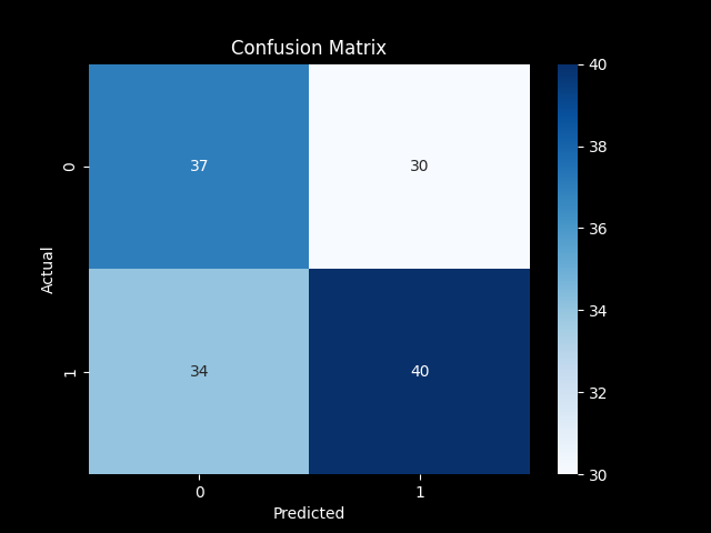
Confusion Matrix
The confusion matrix helps us identify the number of correct and incorrect predictions for both classes (up or down).
Visualizing the Predictions
We can also visualize how well the model’s predictions match the actual stock price movements.
The chart below shows the predicted market direction (up or down) versus the actual closing price of Tesla stock.
plt.figure(figsize=(14,6))
plt.plot(data.index[-len(y_test):], data["Close"][-len(y_test):], label='Close Price')
plt.plot(data.index[-len(y_test):][y_pred == 1], data["Close"][-len(y_test):][y_pred == 1], '^', markersize=10, color='g', label='Predicted Up')
plt.plot(data.index[-len(y_test):][y_pred == 0], data["Close"][-len(y_test):][y_pred == 0], 'v', markersize=10, color='r', label='Predicted Down')
plt.title("Predicted Market Direction vs Close Price")
plt.legend()
plt.savefig("predicted_market_direction.png")
plt.show()
Predicted Market Direction vs Close
This provides a clear visual representation of how the model is performing.
Feature Importance
Finally, we examine which features are the most important in predicting Tesla’s stock direction.
This insight can guide future model improvements and show which aspects of the stock’s behavior contribute most to the predictions.
importances = model.feature_importances_
feat_names = X.columns
plt.barh(feat_names, importances)
plt.title("Feature Importances (Decision Tree)")
plt.xlabel("Importance")
plt.savefig("feature_importances.png")
plt.show()
Feature Importances