
In partnership with

200% Revenue Growth: Be Part of Their Global Expansion

This is a paid advertisement for Med-X’s Regulation CF Offering. Please read the offering circular at https://invest.medx-rx.com/
Fast-growing product expanding globally – invest now
200% revenue growth in five years
Entering 41 international markets, major partnerships
🚀 Your Investing Journey Just Got Better: Premium Subscriptions Are Here! 🚀
It’s been 4 months since we launched our premium subscription plans at GuruFinance Insights, and the results have been phenomenal! Now, we’re making it even better for you to take your investing game to the next level. Whether you’re just starting out or you’re a seasoned trader, our updated plans are designed to give you the tools, insights, and support you need to succeed.
Here’s what you’ll get as a premium member:
Exclusive Trading Strategies: Unlock proven methods to maximize your returns.
In-Depth Research Analysis: Stay ahead with insights from the latest market trends.
Ad-Free Experience: Focus on what matters most—your investments.
Monthly AMA Sessions: Get your questions answered by top industry experts.
Coding Tutorials: Learn how to automate your trading strategies like a pro.
Masterclasses & One-on-One Consultations: Elevate your skills with personalized guidance.
Our three tailored plans—Starter Investor, Pro Trader, and Elite Investor—are designed to fit your unique needs and goals. Whether you’re looking for foundational tools or advanced strategies, we’ve got you covered.
Don’t wait any longer to transform your investment strategy. The last 4 months have shown just how powerful these tools can be—now it’s your turn to experience the difference.
Volatility forecasting is a pillar of risk management, helping investors and financial institutions assess market uncertainty and make informed decisions. Over time, various models have been developed to predict volatility, ranging from traditional econometric approaches like GARCH [1] to the increasingly popular machine learning (ML) techniques [2]. While ML models offer powerful pattern recognition and adaptability, their application in finance requires careful consideration to avoid common pitfalls like look-ahead bias.
Look-ahead bias occurs when a model or strategy inadvertently uses information that would not have been available at the time of making a decision. To set an example, imagine you’re a time-traveling stock trader who goes back to February 2020, knowing about the upcoming COVID-19 pandemic and March market crash. You use this future knowledge to short the market heavily, resulting in millions in profits when March arrives. This scenario illustrates look-ahead bias: making decisions using information that wasn’t actually available at the time, leading to unrealistically positive results (in your backtest) that wouldn’t be achievable in real-world trading.
In this context, we’ll explore how easy it is to unintentionally introduce future information into the training process. Let’s dive into the code.
Hands Down Some Of The Best Credit Cards Of 2025
Pay No Interest Until Nearly 2027 AND Earn 5% Cash Back
1. Data Collection and Preparation
Here, the price data is retrieved from yfinance, and thepandas.DataFrameto be used in the Random Forest model is set up.
import yfinance as yf
import pandas as pd
import numpy as np
import matplotlib.pyplot as plt
from ta.momentum import RSIIndicator
from ta.trend import MACD

# Download historical stock data
ticker = 'AAPL'  # Apple Inc.
data = yf.download(ticker, start="2020-01-01", end="2023-01-01", auto_adjust=False)
data['Returns'] = data['Adj Close'].pct_change()  # Daily returns

# Calculate historical volatility
window = 21  # 21 trading days
data['Volatility'] = data['Returns'].rolling(window=window).std() * np.sqrt(252)  # Annualized volatility

# Feature: 21-day rolling mean (Moving Average)
data['MA_21'] = data['Adj Close'].rolling(window=21).mean()

# Feature: RSI
rsi = RSIIndicator(data['Adj Close'].squeeze(), window=14).rsi()
data['RSI'] = rsi

# Feature: MACD
macd = MACD(data['Adj Close'].squeeze())
data['MACD'] = macd.macd_diff()

# Drop NaN values
data.dropna(inplace=True)
data.columns = data.columns.get_level_values(0)
Explanation:
The features used include daily returns, historical volatility, moving averages of stock prices, and two technical indicators: Relative Strength Index (RSI) and Moving Average Convergence Divergence (MACD).
2. Building and training the Machine Learning Model
A Random Forest Regressor is used to forecast future volatility, with the target variable defined as the volatility one month ahead (volatility shifted by -21). The look-ahead bias in this model is introduced during the data split for training and testing using the train_test_split function from scikit-learn. Specifically, the default setting for the shuffle parameter (shuffle=True) is not changed, which results in random shuffling of the dataset before splitting. This inadvertently allows future information to leak into the training data, leading to a biased model.
Let’s examine how the model’s results change by simply adjusting the value of this parameter.
import numpy as np
import matplotlib.pyplot as plt
from sklearn.model_selection import train_test_split
from sklearn.ensemble import RandomForestRegressor
from sklearn.metrics import mean_squared_error

# Create target variable
data['Future_Volatility'] = data['Volatility'].shift(-21)  # Forecast 21 days ahead

# Drop NaN values
data.dropna(inplace=True)

# Features and target
X = data[['MA_21', 'RSI', 'MACD', 'Volatility']]
y = data['Future_Volatility']

# Function to train model and predict values
def train_and_predict(shuffle_value):
    """Train the model and return actual and predicted values."""
    # Split data with specified shuffle parameter
    X_train, X_test, y_train, y_test = train_test_split(X, y, test_size=0.2, random_state=42, shuffle=shuffle_value)

    # Train Random Forest model
    model = RandomForestRegressor(n_estimators=100, random_state=42)
    model.fit(X_train, y_train)

    # Predict on test data
    y_pred = model.predict(X_test)

    return y_test, y_pred

# Function to evaluate model performance
def evaluate_model(y_test, y_pred):
    """Calculate and return RMSE of the model."""
    rmse = np.sqrt(mean_squared_error(y_test, y_pred))
    return rmse

# Train and evaluate for shuffle=True
y_test_shuffled, y_pred_shuffled = train_and_predict(shuffle_value=True)
rmse_shuffled = evaluate_model(y_test_shuffled, y_pred_shuffled)
print(f"RMSE (Shuffle=True): {rmse_shuffled}")
# Train and evaluate for shuffle=False
y_test_ordered, y_pred_ordered = train_and_predict(shuffle_value=False)
rmse_ordered = evaluate_model(y_test_ordered, y_pred_ordered)
print(f"RMSE (Shuffle=False): {rmse_ordered}")
Explanation:
Here we train the RF model with the two shuffle values: shuffle=Trueand shuffle=False.
3. Evaluating the Machine Learning Model
# Function to plot actual vs predicted values
def plot_actual_vs_predicted(y_test, y_pred, shuffle_value, ax):
    """Plot the actual vs predicted values as a scatter plot."""
    # Plot actual vs. predicted values
    ax.scatter(y_test, y_pred, alpha=0.5)

    # Plot the ideal line (45-degree line)
    ax.plot([min(y_test), max(y_test)], [min(y_test), max(y_test)], color='red', linestyle='--', linewidth=2)  # Ideal line

    # Set titles and labels
    ax.set_title(f"Shuffle={shuffle_value}", fontsize=16, fontweight='bold')
    ax.set_xlabel("Actual Volatility", fontsize=14)
    ax.set_ylabel("Predicted Volatility", fontsize=14)

    # Improve ticks and grid
    ax.tick_params(axis='both', which='major', labelsize=12)
    ax.grid(True, linestyle='--', alpha=0.7)

# Create subplots
fig, axes = plt.subplots(1, 2, figsize=(14, 6))  # Two subplots in one row

# Plot for shuffle_value=True
plot_actual_vs_predicted(y_test_shuffled, y_pred_shuffled, shuffle_value=True, ax=axes[0])
# Plot for shuffle_value=False
plot_actual_vs_predicted(y_test_ordered, y_pred_ordered, shuffle_value=False, ax=axes[1])

# Adjust layout for clarity
plt.tight_layout()
plt.show()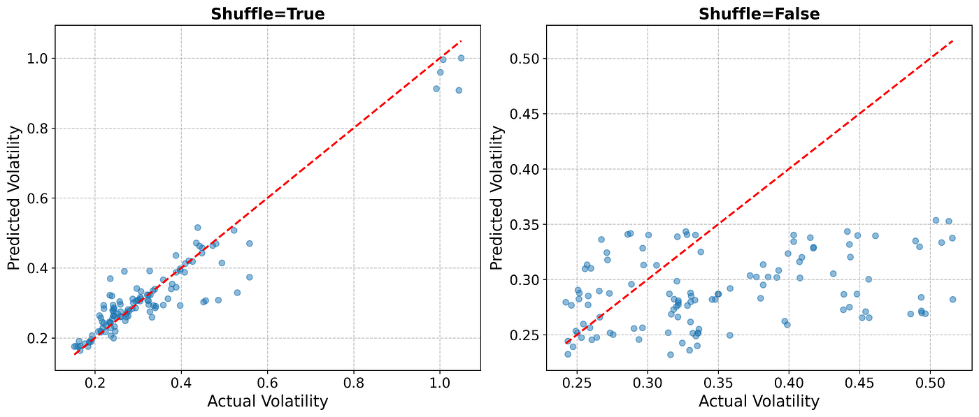
Impact of Data Shuffling on Volatility Forecasting: predicted vs. actual volatility when using Random Forest with shuffle=True (left) and shuffle=False (right). The red dashed line represents an ideal prediction. Notice how shuffling introduces look-ahead bias, leading to overly optimistic results.
The figure above highlights the impact of data shuffling on volatility forecasting with Random Forest. When shuffle=True (left plot), the predicted values appear closely aligned with actual volatility, suggesting strong model performance. However, this is misleading due to look-ahead bias. In contrast, when shuffle=False (right plot), the predictions deviate significantly from actual values, reflecting a more realistic out-of-sample performance. This is further quantified by the 70% increase in Mean Squared Error (MSE) in the test set (on average), demonstrating how improper data handling can severely distort forecasting accuracy.
Another way of looking at the difference is plotting the target and predicted time series, like it was done in the original post.
# Function to plot time-series
def plot_series(y_test, y_pred, title, ax):
    """Plot actual vs predicted volatility in a given subplot."""
    ax.plot(y_test.values, label='Actual Volatility', color='blue')
    ax.plot(y_pred, label='Predicted Volatility', color='red')
    ax.set_title(title, fontsize=16, fontweight='bold')
    ax.legend()
    ax.grid(True, linestyle='--', alpha=0.7)
    ax.set_xlabel("Time", fontsize=14)
    ax.set_ylabel("Volatility", fontsize=14)
    ax.tick_params(axis='both', labelsize=12)


# Create figure with two subplots
fig, axes = plt.subplots(1, 2, figsize=(14, 6))

# Plot for shuffle=True
plot_series(y_test_shuffled, y_pred_shuffled, "Shuffle=True (Biased)", axes[0])

# Plot for shuffle=False
plot_series(y_test_ordered, y_pred_ordered, "Shuffle=False (Realistic)", axes[1])

# Adjust layout
plt.tight_layout()
plt.show()
Comparison of Actual vs Predicted Volatility: The left plot shows the model performance with shuffle=True, leading to a look-ahead bias. The right plot shows the results with shuffle=False, reflecting a more realistic, unbiased forecasting approach.
As seen in the figure, there is a significant difference between introducing a look-ahead bias (left) and simulating a real-life scenario (right). The plot on the left shows predictions vs. target volatility values from the test set, where the data comes from a shuffled dataset (shuffle=True). Here, the x-axis doesn’t represent time but rather an arbitrary index. On the right, with shuffle=False, the model respects the natural order of time, and while the predictions are less accurate, the x-axis accurately reflects time, which mirrors real-world forecasting conditions.
4. Final Remarks
Setting shuffle=True in time series forecasting introduces look-ahead bias because it randomly shuffles the dataset before splitting it into training and test sets. This means that future data points can end up in the training set while earlier data points are in the test set.
Since time series data has a natural temporal order (where past values influence future values), shuffling disrupts this order and allows the model to learn patterns that include information from the future — something that would be impossible in real-world forecasting. As a result, the model appears to perform much better than it actually would in a true out-of-sample scenario, leading to overly optimistic results that won’t hold in live trading or real applications.
Forecasting volatility of financial assets is undoubtedly a challenging task, particularly when predicting over longer time horizons [3]. The inherent unpredictability of markets, coupled with the complexity of capturing the right features, makes it difficult to achieve consistent accuracy. Moreover, when applying machine learning models to volatility forecasting, it’s crucial to be vigilant about the potential leakage of future data during the training process. Even small slips, such as unintentional shuffling of data, can lead to inflated performance metrics and undermine the reliability of the model in real-world scenarios.
Disclaimer: here we use yfinance for easy access to financial data, but we do not recommend using yfinance datasets for backtesting, as it displays other types of look-ahead bias.
References:
[1] Engle, R. F. Autoregressive Conditional Heteroskedasticity with Estimates of the Variance of United Kingdom Inflation. Econometrica, 50(4), 987–1007 (1982).
[2] Zhang, L., Xie, L., & Zheng, Y. Forecasting financial volatility with deep learning. Journal of Computational Finance, 23(2), 1–22 (2019).
[3] Andersen, T. G., & Bollerslev, T. Deutsche mark–dollar volatility: Intraday activity patterns, macroeconomic announcements, and longer run dependencies. Journal of Finance, 53(1), 219–265 (1998).