Elon Dreams, Mode Mobile Delivers

As Elon Musk said, “Apple used to really bring out products that would blow people’s minds.”

Thankfully, a new smartphone company is stepping up to deliver the mind-blowing moments we've been missing.

Turning smartphones from an expense into an income stream, Mode has helped users earn an eye-popping $325M+ and seen an astonishing 32,481% revenue growth rate over three years.

They’ve just been granted the stock ticker $MODE by the Nasdaq—and the share price changes soon.

Invest before 5/1 price change.

_{*An intent to IPO is no guarantee that an actual IPO will occur. Please read the offering circular and related risks at invest.modemobile.com.
*The Deloitte rankings are based on submitted applications and public company database research.}

🚀 Your Investing Journey Just Got Better: Premium Subscriptions Are Here! 🚀

It’s been 4 months since we launched our premium subscription plans at GuruFinance Insights, and the results have been phenomenal! Now, we’re making it even better for you to take your investing game to the next level. Whether you’re just starting out or you’re a seasoned trader, our updated plans are designed to give you the tools, insights, and support you need to succeed.

Here’s what you’ll get as a premium member:

• Exclusive Trading Strategies: Unlock proven methods to maximize your returns.

• In-Depth Research Analysis: Stay ahead with insights from the latest market trends.

• Ad-Free Experience: Focus on what matters most—your investments.

• Monthly AMA Sessions: Get your questions answered by top industry experts.

• Coding Tutorials: Learn how to automate your trading strategies like a pro.

• Masterclasses & One-on-One Consultations: Elevate your skills with personalized guidance.

Our three tailored plans—Starter Investor, Pro Trader, and Elite Investor—are designed to fit your unique needs and goals. Whether you’re looking for foundational tools or advanced strategies, we’ve got you covered.

Don’t wait any longer to transform your investment strategy. The last 4 months have shown just how powerful these tools can be—now it’s your turn to experience the difference.

👉 Explore Premium Plans Now

Imagine financial markets as a living, breathing organism, constantly shifting, evolving, and responding to the collective pulse of global economic activities. Each moment carries its own unique energy, its distinct personality. What appears calm today might transform into a volatile storm tomorrow. This intricate dance of market behavior is precisely what makes market regime analysis so fascinating.

Understanding Market Regimes: Beyond Simple Numbers

A market regime is far more than a mere statistical snapshot. It’s a comprehensive narrative of market psychology, capturing the collective emotions, fears, and expectations of investors at a specific moment in time. Think of it as a financial mood ring that reveals the underlying sentiment driving market movements.

Traditionally, investors have sought to understand these market transformations through complex and often prohibitively expensive analyses. Our approach offers a systematic method that breaks down this complexity into manageable, quantifiable components.

The gold standard of business news

Morning Brew is transforming the way working professionals consume business news.

They skip the jargon and lengthy stories, and instead serve up the news impacting your life and career with a hint of wit and humor. This way, you’ll actually enjoy reading the news—and the information sticks.

Best part? Morning Brew’s newsletter is completely free. Sign up in just 10 seconds and if you realize that you prefer long, dense, and boring business news—you can always go back to it.

Join 4.3 Million Readers Now

The Methodology: Unraveling Market Complexity

Our analysis rests on three fundamental pillars: data collection, volatility calculation, and regime classification. Each of these steps is crucial in transforming raw market data into meaningful insights.

Data Collection: Painting the Financial Canvas

We begin by capturing two critical market indicators: the S&P 500 and the VIX Index. The S&P 500 provides a panoramic view of the U.S. stock market, while the VIX acts as a thermometer measuring market volatility and investor fear.

Our analysis spans a three-year window (a carefully chosen timeframe that balances historical depth with current market relevance). This isn’t an arbitrary decision, but a strategic approach to capturing meaningful market trends while maintaining analytical currency.

Volatility Calculation: Peering Beyond the Obvious

This is where our methodology becomes truly sophisticated. Instead of relying on simple volatility measures, we employ the Yang-Zhang volatility estimation method(an advanced statistical model that captures multiple dimensions of market volatility).

The Yang-Zhang method is revolutionary in its approach. It doesn’t settle for a single perspective but deconstructs volatility into specific components: overnight volatility, open-to-close volatility, and an innovative calculation considering price movements between highs and lows. Imagine it as a financial prism that breaks down market movement into its fundamental spectrum.

This approach allows us to understand not just how much the market moves but also the nuanced reasons behind those movements. Volatility transforms from a cold number into a narrative of financial behavior.

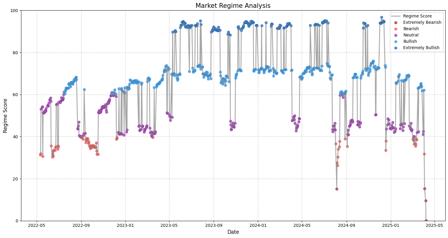
Regime Classification: Translating Numbers into Narratives

Our classification system goes beyond simple bullish or bearish categorizations. We create a five-state spectrum that captures the market’s emotional nuances:

From “Extremely Bearish” to “Extremely Bullish,” with neutral states in between, each classification represents a distinct market mood. It’s like creating an emotional map of financial landscapes.

The algorithm carefully weights multiple factors: historical volatility, VIX ratio and volatility trends. Each component contributes a unique perspective, like musicians in an orchestra creating a complex financial symphony.

Beyond the Numbers: Interpretation and Context

The most critical understanding is that no model can predict the future with absolute certainty. Our market regime analysis is a tool for comprehension, not a crystal ball. It provides a structured perspective for informed decision-making, but it does not guarantee outcomes.

The most successful investors are those who combine this quantitative analysis with fundamental research, a broader understanding of economic contexts, and, most importantly, a critical and adaptable mindset.

import yfinance as yf
import pandas as pd
import numpy as np
import matplotlib.pyplot as plt
from datetime import datetime, timedelta

class MarketRegimeAnalyzer:
    def __init__(self, start_date=None, end_date=None):
        """
        Initialize Market Regime Analyzer

        Args:
            start_date (str, optional): Start date for analysis. Defaults to 3 years ago.
            end_date (str, optional): End date for analysis. Defaults to today.
        """
        # Set default date range if not provided
        if start_date is None:
            start_date = (datetime.now() - timedelta(days=3*365)).strftime('%Y-%m-%d')
        if end_date is None:
            end_date = datetime.now().strftime('%Y-%m-%d')

        self.start_date = start_date
        self.end_date = end_date

        # Tickers for analysis
        self.indices = {
            'SPX': '^GSPC',
            'VIX': '^VIX'
        }

        # Data storage
        self.data = {}

    def fetch_data(self):
        """
        Fetch historical data for specified indices

        Returns:
            MarketRegimeAnalyzer: Self with fetched data
        """
        for name, ticker in self.indices.items():
            try:
                # Download data using yfinance with explicit auto_adjust
                # Wrap single ticker in a list to avoid previous error
                df = yf.download([ticker], start=self.start_date, end=self.end_date, auto_adjust=True)

                # If DataFrame has multi-level columns, flatten them
                if isinstance(df.columns, pd.MultiIndex):
                    df.columns = [f'{col[0]}_{col[1]}' for col in df.columns]

                # Ensure numeric columns for calculations
                numeric_columns = ['Open', 'High', 'Low', 'Close']
                for suffix in ['', '_Open', '_High', '_Low', '_Close']:
                    for col in [f'{suffix}' for suffix in numeric_columns]:
                        if col in df.columns:
                            df[col] = pd.to_numeric(df[col], errors='coerce')

                # Add column with ticker name
                df['Ticker'] = name
                self.data[name] = df

            except Exception as e:
                print(f"Error fetching data for {name}: {e}")
                # Verbose error tracking
                import traceback
                traceback.print_exc()

        return self

    def calculate_yang_zhang_volatility(self, ohlc_data, window=21):
        """
        Calculate Yang-Zhang volatility

        Args:
            ohlc_data (pd.DataFrame): OHLC price data
            window (int, optional): Rolling window. Defaults to 21.

        Returns:
            pd.Series: Annualized volatility
        """
        # Identify correct column names
        open_col = [col for col in ohlc_data.columns if 'Open' in col][0]
        high_col = [col for col in ohlc_data.columns if 'High' in col][0]
        low_col = [col for col in ohlc_data.columns if 'Low' in col][0]
        close_col = [col for col in ohlc_data.columns if 'Close' in col][0]

        # Ensure data integrity
        ohlc_data = ohlc_data.dropna(subset=[open_col, high_col, low_col, close_col])

        # Parameters
        k = 0.34  # Standard Yang-Zhang parameter

        # Calculate overnight returns
        overnight_returns = np.log(ohlc_data[open_col] / ohlc_data[close_col].shift(1))
        overnight_vol_sq = overnight_returns.rolling(window=window).var()

        # Open-to-close volatility
        open_close_returns = np.log(ohlc_data[close_col] / ohlc_data[open_col])
        open_close_vol_sq = open_close_returns.rolling(window=window).var()

        # Rogers-Satchell volatility
        rs_terms = (np.log(ohlc_data[high_col] / ohlc_data[open_col]) *
                    np.log(ohlc_data[high_col] / ohlc_data[close_col]) +
                    np.log(ohlc_data[low_col] / ohlc_data[open_col]) *
                    np.log(ohlc_data[low_col] / ohlc_data[close_col]))

        rs_vol_sq = rs_terms.rolling(window=window).mean()

        # Yang-Zhang volatility
        yz_vol_sq = overnight_vol_sq + k * rs_vol_sq + (1 - k) * open_close_vol_sq
        yz_vol = np.sqrt(yz_vol_sq) * np.sqrt(252)  # Annualized

        return yz_vol

    def detect_market_regime(self):
        """
        Detect market regime based on volatility and VIX metrics

        Returns:
            pd.DataFrame: Market regime score and classification
        """
        if not self.data:
            self.fetch_data()

        # Verify data was fetched
        if not self.data or 'SPX' not in self.data or 'VIX' not in self.data:
            raise ValueError("Failed to fetch market data. Please check internet connection and ticker symbols.")

        # Prepare S&P 500 and VIX data
        # Find the correct close column
        spx_close_col = [col for col in self.data['SPX'].columns if 'Close' in col][0]
        vix_close_col = [col for col in self.data['VIX'].columns if 'Close' in col][0]

        sp500 = self.data['SPX']
        vix = self.data['VIX']

        # Calculate volatility
        sp500_volatility = self.calculate_yang_zhang_volatility(sp500)

        # Calculate volatility metrics with safeguards
        sp500_vol_median = sp500_volatility.rolling(window=252).median()

        # Calculate VIX ratio
        vix_median = vix[vix_close_col].rolling(window=21).median()
        vix_ratio = vix[vix_close_col] / vix_median

        # Regime components calculation with robust handling
        def safe_normalize(series):
            """Safely normalize a series to 0-1 range"""
            min_val = series.min()
            max_val = series.max()
            range_val = max_val - min_val

            # Avoid division by zero
            if range_val == 0:
                return pd.Series(0.5, index=series.index)

            return 1 - ((series - min_val) / range_val)

        # Calculate regime score components
        vol_score = safe_normalize(sp500_volatility)

        # VIX Ratio Score
        vix_ratio_score = safe_normalize(vix_ratio)

        # Additional components
        vol_median_score = (sp500_vol_median > sp500_volatility).astype(float)
        vix_ratio_threshold_score = (vix_ratio < 1).astype(float)

        # Combine components
        regime_score = (
            0.3 * vol_score +
            0.2 * vol_median_score +
            0.3 * vix_ratio_score +
            0.2 * vix_ratio_threshold_score
        ) * 100

        # Classify regime
        def classify_regime(score):
            if pd.isna(score):
                return 'Insufficient Data'
            elif score <= 20:
                return 'Extremely Bearish'
            elif score <= 40:
                return 'Bearish'
            elif score <= 60:
                return 'Neutral'
            elif score <= 80:
                return 'Bullish'
            else:
                return 'Extremely Bullish'

        # Create DataFrame with results
        regime_df = pd.DataFrame({
            'Score': regime_score,
            'Classification': regime_score.apply(classify_regime)
        }, index=sp500.index)

        return regime_df

    def visualize_regime(self, regime_df):
        """
        Visualize market regime analysis

        Args:
            regime_df (pd.DataFrame): Market regime DataFrame
        """
        plt.figure(figsize=(15, 8))

        # Color mapping for different regimes
        color_map = {
            'Extremely Bearish': '#B21818',
            'Bearish': '#EF5350',
            'Neutral': '#9C27B0',
            'Bullish': '#2196F3',
            'Extremely Bullish': '#1565C0',
            'Insufficient Data': '#9E9E9E'
        }

        # Clean out NaN values
        regime_df_clean = regime_df.dropna()

        # Plot regime score
        plt.plot(regime_df_clean.index, regime_df_clean['Score'],
                 linewidth=2,
                 color='gray',
                 alpha=0.7,
                 label='Regime Score')

        # Scatter plot with color-coded points
        for regime in color_map:
            mask = regime_df_clean['Classification'] == regime
            subset = regime_df_clean[mask]
            if not subset.empty:
                plt.scatter(subset.index,
                            subset['Score'],
                            c=color_map[regime],
                            label=regime,
                            alpha=0.7)

        plt.title('Market Regime Analysis', fontsize=15)
        plt.xlabel('Date', fontsize=12)
        plt.ylabel('Regime Score', fontsize=12)
        plt.ylim(0, 100)
        plt.legend()
        plt.grid(True, linestyle='--', alpha=0.7)
        plt.tight_layout()
        plt.show()

    def run_analysis(self):
        """
        Run complete market regime analysis

        Returns:
            pd.DataFrame: Market regime results
        """
        regime_df = self.detect_market_regime()
        self.visualize_regime(regime_df)
        return regime_df

# Example usage
if __name__ == "__main__":
    # Initialize and run analysis
    analyzer = MarketRegimeAnalyzer()
    results = analyzer.run_analysis()

    # Print most recent regime details
    print("\nMost Recent Market Regime:")
    most_recent = results.dropna().tail(1)
    print(most_recent)

    # Print summary statistics
    print("\nRegime Summary Statistics:")
    summary_stats = results.groupby('Classification').describe()
    print(summary_stats)

    # Additional insights
    print("\nRegime Distribution:")
    regime_distribution = results['Classification'].value_counts(normalize=True) * 100
    print(regime_distribution)

A Final Reflection

Financial markets are complex ecosystems filled with subtle interactions and changing dynamics. Understanding their regimes is not just about numbers, it’s about comprehending the dance of information, collective psychology, and global economic currents.

Our methodology doesn’t aim to simplify this complexity but to offer a clearer window through which to observe it. It’s an invitation to look beyond surface-level data and dive into the rich narrative that markets tell us every day.