Market Timing Beats Time in the Market (At Least Since 1871)

Exciting News: We Are Launching A Waitlist!

Last week I sent you all an email that starting from September, we’re introducing paid subscriptions to bring you even more value. Free users will still have access to market insights and weekly news, but paid subscribers will get:

• Exclusive trading strategies used by me and my team

• The Research Paper Analysis And Strategies Built Upon Them

• Ad-free content for a seamless reading experience

• AMA sessions to get your questions answered directly

As we expand and bring on more team members to improve this publication, we need to cover rising costs. Please let us know if you’re interested in these updates by filling out this Waitlist Google Form. 

Your feedback is key to shaping our future!

🗣️ Stock Market Today: As US rate cuts near, economic 'soft-landing' odds could dictate stock performance

Investors are increasingly focusing on upcoming economic data as they assess whether the "soft landing" narrative that has driven U.S. stocks in 2024 can continue, especially with interest rate cuts almost certain. Federal Reserve Chair Jerome Powell signaled at the Jackson Hole conference that the time is right to start lowering rates, likely beginning with a 25 basis-point cut in September. While the market reacted positively, concerns remain about whether the rate cuts indicate underlying economic worries. Historically, stocks perform better when rate cuts occur during periods of resilient growth rather than during sharp economic slowdowns.

The outlook for stocks remains uncertain, with key data points like upcoming inflation reports potentially influencing market sentiment. Investors are cautious about whether rate cuts are driven by moderating inflation or a weakening labor market, with the latter scenario potentially dampening enthusiasm. Additionally, elevated stock valuations and the historical weakness of September's market performance contribute to a volatile trading environment. The tight presidential race between Vice President Kamala Harris and former President Donald Trump may also add to the uncertainty as the November election approaches.

Stay informed with today's rundown:

Today, we delve into the “Market Timing Beats Time in the Market (At Least Since 1871)”👇

"Everyone agrees that it’s appropriate to divide the space of a portfolio between different asset classes," i.e., dividing your portfolio between different asset classes (e.g., 60% stocks and 40% bonds). However, it remains controversial to divide the time of your portfolio between different asset classes as market conditions change, also known as market timing. It is an alternative to maintaining a singular asset allocation over time (or changing your asset allocation in response to non-market conditions, like your age). Despite its poor reputation, the data show that market timing beats time in the market (at least since 1871).

The premise of the strategies discussed in this post is simple: things that are trending down tend to keep trending down, and vice versa. I won't get into why this is true (though as I've written about previously, investors aren't rational, and tend to panic sell during a down trend and pile in during an up trend), just that following market trends has been beneficial since 1871. It's the premise behind trend following, which has been practiced for hundreds of years. (Disclaimer: these strategies are not new and not my own).

The scope of this post is the US market, specifically the S&P 500 index and the 10-Year Treasury Bond (GS10). Historical data was obtained from Professor Shiller (most well known for CAPE). Total return (including dividends) is used for the S&P 500 and monthly returns for 10-Year Treasury Bonds (Long Government Bond pre-1953) are calculated using Professor Damodaran's methodology (which isn't 100% correct, but is close enough). The strategies are rebalanced at the first of every month. And by the way, I'm only calculating Sharpe ratio after 1934 because the risk free rate I'm using is the yield on the 3-month Treasury Bill.

The two strategies both use a simple moving average (SMA) and are described below:

• SMA(10) - When the price of the S&P 500 index closes below it's 10-month (200-day) SMA, sell the S&P 500 index (stocks) and buy the 10-Year Treasury Bond (bonds). Keep holding bonds until the price of the S&P closes above it's 10-month SMA.

• SMA Cross - When the 50-day (2.5-month) SMA of the S&P closes below it's 200-day SMA (also called the death cross), sell stocks and buy bonds. Keep holding bonds until the 50-day SMA crosses above the 200-day SMA (also called the golden cross).

These two strategies will be compared against buying and holding each of the following asset allocations:

• 100% stocks (again, total return of the S&P 500 index, including dividends)

• 100% bonds (10-Year Treasury Bond)

• 63% stocks & 37% bonds (it turns out that since 1871, both of the SMA strategies are in stocks about 63% of the time and in bonds about 37% of the time, so I thought this would be a more interesting comparison)

Obviously, these strategies have worked very well historically. The returns by decade are shown below.

The only decade where the S&P 500 Total Return outperformed both market timing strategies was the 1990s. Below are charts showing how the CAGR, Sharpe ratio, and maximum drawdowns (from starting year to 2017) change as the starting year changes.

These charts tell the same story, with the market timing strategies leading the pack regardless of the starting year. The max drawdown chart is interesting because you can clearly see recessions and how each strategy performed by the magnitude of the drop.

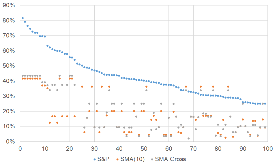
Speaking of drawdowns, the 100 largest drawdowns of the S&P 500 Total Return and the corresponding drawdowns of the market timing strategies are shown below.

The data depicted was not organized for individual recessions, so there is some overlap and misrepresentation. The raw data with associated dates is here.

Saving the best for last, the base rates for the strategies are below.

These base rates tell you what % of time each strategy has resulted in a positive (1-, 3-, 5-, or 10-year) CAGR. For example, for 3.4% of the rolling 10-year time periods between 1871 and 2017, you would have lost money (return less than 0%) by being invested in the S&P 500. Or, there was an 89.9% chance that you'd have a positive return on a 10-Year Treasury Bond during any given year between 1871 and 2017.

Base rates can be very helpful psychologically; knowing how often a 3-year losing streak has happened in the past can provide a frame of reference when trying to decide to change strategies or stick with it.

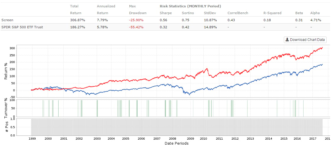
Using more powerful tools, these strategies can be tested and implemented with more recent data. Below are results for both strategies using SPY and IEF from 1999 to present. (I know that IEF was only introduced in 2002, but the site I use has extended the price for this and many other ETFs backward to maximize usefulness in backtesting).

Switching out ETFs (e.g., SHY to short the market instead of IEF, just going to cash, using a more bullish ETF), using exponential moving averages instead of SMAs, combining market timing indicators, implementing these timing rules into other portfolios (stock or ETF), and many more permutations are all things to explore.

Future posts include more market indicators as well as economic indicators (such as unemployment rate, and how well it's worked since 1948 when it was first published) that can be used to help inform your investment decisions.

I recommend further reading by people smarter than me, if you're interested.

You can save up to 100% on a Tradingview subscription with my refer-a-friend link. When you get there, click on the Tradingview icon on the top-left of the page to get to the free plan if that’s what you want.