Mastering Merton’s Jump-Diffusion Model for Trading Insights

Marketing ideas for marketers who hate boring

The best marketing ideas come from marketers who live it. That’s what The Marketing Millennials delivers: real insights, fresh takes, and no fluff. Written by Daniel Murray, a marketer who knows what works, this newsletter cuts through the noise so you can stop guessing and start winning. Subscribe and level up your marketing game.

Sign Up Free

🚀 Your Investing Journey Just Got Better: Premium Subscriptions Are Here! 🚀

It’s been 4 months since we launched our premium subscription plans at GuruFinance Insights, and the results have been phenomenal! Now, we’re making it even better for you to take your investing game to the next level. Whether you’re just starting out or you’re a seasoned trader, our updated plans are designed to give you the tools, insights, and support you need to succeed.

Here’s what you’ll get as a premium member:

• Exclusive Trading Strategies: Unlock proven methods to maximize your returns.

• In-Depth Research Analysis: Stay ahead with insights from the latest market trends.

• Ad-Free Experience: Focus on what matters most—your investments.

• Monthly AMA Sessions: Get your questions answered by top industry experts.

• Coding Tutorials: Learn how to automate your trading strategies like a pro.

• Masterclasses & One-on-One Consultations: Elevate your skills with personalized guidance.

Our three tailored plans—Starter Investor, Pro Trader, and Elite Investor—are designed to fit your unique needs and goals. Whether you’re looking for foundational tools or advanced strategies, we’ve got you covered.

Don’t wait any longer to transform your investment strategy. The last 4 months have shown just how powerful these tools can be—now it’s your turn to experience the difference.

👉 Explore Premium Plans Now

In this article, we will dissect Merton’s model. We will learn how to simulate these price jumps in Python, analyze their profound impact on return distributions, and use the model to price options, ultimately generating the classic “ volatility smile “ that is characteristic of markets influenced by jump risk.

The Anatomy of a Jump-Diffusion Process

The Merton model extends the Geometric Brownian Motion (GBM) framework by adding a component that explicitly models jumps. The stochastic differential equation (SDE) for the asset price

​ looks like this:

This equation might seem complex, but it’s really just two ideas stitched together.

Part 1: The Diffusion Component

This is the standard GBM process describing the “normal” behavior of the stock price between jumps.

• μ is the expected return of the asset.

• σ is the constant volatility of the diffusion part.

• \(W_t\)​ is the familiar Wiener process or Brownian motion.

• The drift term μ is adjusted by subtracting λk. This is a crucial compensator. It ensures that the overall expected return of the asset remains μ, even after we add the jumps. We’ll define λ and k in a moment.

What Smart Investors Read Before the Bell Rings

Clickbait headlines won’t grow your portfolio. That’s why over 1M investors — including Wall Street insiders — start their day with The Daily Upside. Founded by investment bankers and journalists, it cuts through the noise with clear insights on business, markets, and the economy. Stop guessing and get smarter every morning.

Subscribe free today.

The Jump Component

This is the new and exciting part that introduces the discontinuous leaps.

• \(dN_t\)​​ is a Poisson process with an intensity or arrival rate of λ. This process governs if a jump happens. In any small time interval dt, \(dN_t\)​​ can be either 1 (a jump occurs) with probability λdt, or 0 (no jump occurs) with probability 1−λdt. λ represents the average number of jumps per year.

• \(J_t\)​​ is a random variable representing the size of the jump. When a jump occurs, the price moves from \(S_t\)​​ to \(S_t\)\(J_t\)​. If \(J_t\)​ ​= 1.1, it’s a 10% jump up; if \(J_t\)​ ​= 0.8, it’s a 20% jump down.

• The jump size \(J_t\) is typically assumed to be log-normally distributed, meaning ln(\(J_t\)​) follows a normal distribution with mean \(μ_j\)​ and standard deviation \(σ_j\)​​.

• \(μ_j\)​ ​: The average log-jump size.

• \(σ_j\)​​ : The volatility of the log-jump size.

• Finally, k = E[\(J_t\)​​ ​− 1] = \(e^{μ_j+0.5σ_j²}-1\)​​ is the expected relative jump size. This is the value used to adjust the drift in the diffusion part, ensuring the model is internally consistent.

In short, the Merton model describes a world where the asset price mostly drifts and diffuses according to GBM but is intermittently shocked by jumps of random size that arrive at random times.

Simulating a World of Jumps in Python

To truly grasp the model’s behavior, we must simulate it. Our simulation needs to handle both the continuous and discrete parts of the process. For each time step, we’ll first calculate the standard diffusion and then check if a jump occurred. If it did, we’ll add its effect.

Let’s define our parameters and build the simulation function.

import numpy as np
import matplotlib.pyplot as plt
import seaborn as sns
from scipy.stats import norm

# Set plotting style
sns.set_theme(style="whitegrid")

# Model Parameters
S0 = 100.0      # Initial asset price
mu = 0.05       # Expected return
sigma = 0.2     # Volatility of the diffusion part

# Jump Parameters
lambda_ = 0.5   # Jump intensity (average 0.5 jumps per year)
mu_j = -0.1     # Mean of log-jump size
sigma_j = 0.3   # Volatility of log-jump size

# Simulation Parameters
T = 1.0         # Time to maturity (1 year)
N = 252         # Number of time steps in a year
M = 1000        # Number of simulations (paths)
dt = T / N      # Size of each time step

# Calculate the drift compensator k
k = np.exp(mu_j + 0.5 * sigma_j**2) - 1

def merton_jump_diffusion_simulation(S0, mu, sigma, lambda_, mu_j, sigma_j, T, N, M):
    """
    Simulates asset price paths using the Merton jump-diffusion model.
    """
    # Calculate the adjusted drift for the diffusion part
    drift = mu - lambda_ * (np.exp(mu_j + 0.5 * sigma_j**2) - 1)
    
    # Initialize array for asset paths
    S = np.zeros((N + 1, M))
    S[0] = S0
    
    for i in range(1, N + 1):
        # Generate random numbers for diffusion and jumps
        Z = np.random.normal(0, 1, M)
        # Poisson process determines the number of jumps in the interval dt
        N_jumps = np.random.poisson(lambda_ * dt, M)
        
        # Calculate the jump sizes if jumps occur
        # Sum of log-normals is not log-normal, so we simulate each jump
        total_jump_size = np.zeros(M)
        for j in range(M):
            if N_jumps[j] > 0:
                # Sum of individual log-jump sizes
                jump_sizes = np.random.normal(mu_j, sigma_j, N_jumps[j])
                total_jump_size[j] = np.sum(jump_sizes)
        
        jump_factor = np.exp(total_jump_size)

        # Calculate the price for the current time step
        S[i] = S[i-1] * np.exp((drift - 0.5 * sigma**2) * dt + sigma * np.sqrt(dt) * Z) * jump_factor
        
    return S

# Run the simulation
S_paths = merton_jump_diffusion_simulation(S0, mu, sigma, lambda_, mu_j, sigma_j, T, N, M)

# --- Plotting the results ---
plt.figure(figsize=(12, 7))
plt.plot(S_paths[:, :10]) # Plot first 10 paths
plt.title('Merton Jump-Diffusion: Sample Asset Paths', fontsize=16)
plt.xlabel('Time Steps')
plt.ylabel('Asset Price')
plt.grid(True)
plt.show()

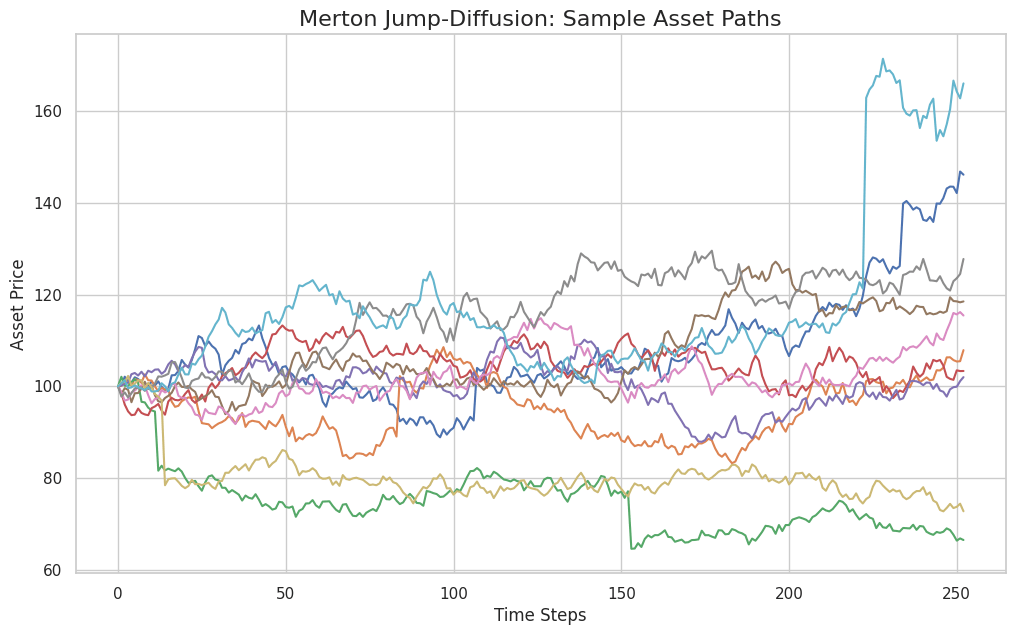
The resulting plot is striking. We see paths that mostly resemble the familiar random walk of Geometric Brownian Motion, but they are punctuated by sudden, sharp vertical leaps. These are our simulated jumps in action, providing a much more realistic picture of how many asset prices actually behave.

The Telltale Signature: Fatter Tails

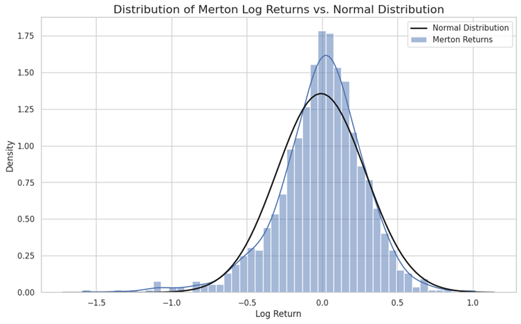
The most significant impact of adding jumps to a model is on the distribution of returns. While the Heston model created fatter tails than a normal distribution, the Merton model takes this to another level. The possibility of large, instantaneous price shocks dramatically increases the probability of extreme returns.

Let’s analyze the distribution of our simulated returns and compare it to a normal distribution.

# --- This code continues from the previous block ---
# --- You should have S_paths available in your environment ---

# Calculate log returns from the simulated asset paths
log_returns = np.log(S_paths[-1] / S0)

# Calculate statistics
mean_return = np.mean(log_returns)
std_return = np.std(log_returns)
skewness = np.mean(((log_returns - mean_return) / std_return)**3)
kurtosis = np.mean(((log_returns - mean_return) / std_return)**4) # Excess kurtosis is this minus 3

print(f"--- Merton Model Return Statistics ---")
print(f"Skewness: {skewness:.4f}")
print(f"Kurtosis: {kurtosis:.4f}")

# Plot the distribution
plt.figure(figsize=(12, 7))
sns.histplot(log_returns, kde=True, bins=50, stat='density', label='Merton Returns')

# Overlay a normal distribution with the same mean and std dev for comparison
xmin, xmax = plt.xlim()
x = np.linspace(xmin, xmax, 100)
p = norm.pdf(x, mean_return, std_return)
plt.plot(x, p, 'k', linewidth=2, label='Normal Distribution')

plt.title('Distribution of Merton Log Returns vs. Normal Distribution', fontsize=16)
plt.xlabel('Log Return')
plt.ylabel('Density')
plt.legend()
plt.show()

The results are clear. The kurtosis value are significantly higher than 3, indicating extremely fat tails. The plot visually confirms this: the central peak of the Merton distribution is higher and narrower, and the tails are much fatter than the normal distribution. This tells us that the model correctly predicts a world where small day-to-day movements are common, but catastrophic (or euphoric) price jumps are a distinct possibility.

Pricing Options with Merton’s Formula

One of the most elegant aspects of Merton’s model is its option pricing formula. Instead of deriving a completely new, complex formula from scratch, Merton showed that the price of a jump-diffusion option is a weighted average of standard Black-Scholes prices.

The intuition is as follows: over the life of the option, there could be zero jumps, one jump, two jumps, and so on. The probability of having exactly n jumps is given by the Poisson distribution. The Merton price is therefore the sum of the prices of Black-Scholes options, weighted by the probability of that number of jumps occurring.

The formula is:

Where:

• The fraction term is the Poisson probability of n jumps.

• \(C_{BS}\) is the Black-Scholes call price.

• The parameters for the Black-Scholes formula are adjusted to account for the impact of the n jumps:

• λ′ = λ (1 + k): The risk-neutral jump intensity.

• \(σ_n²=σ²+n\frac{σ_J²}{T}\)​: The total variance, which is the base diffusion variance plus the variance contributed by n jumps.

• \(r_n=r-λK+n\frac{ln(1+K)}{T}\)​: The adjusted risk-free rate.

In practice, we can’t sum to infinity. However, the Poisson probability quickly becomes negligible for large n, so we can get a very accurate price by truncating the sum after a reasonable number of terms (e.g., 10–15).

# --- This code builds upon the previous blocks ---

# Option and Market Parameters
K = 100.0       # Strike price
r = 0.05        # Risk-free rate
# We reuse the other Merton & simulation parameters (S0, sigma, etc.)

# --- Analytical Pricer for Merton Model ---

# Black-Scholes helper function (from previous article)
def black_scholes_call(S, K, T, r, sigma):
    d1 = (np.log(S / K) + (r + 0.5 * sigma**2) * T) / (sigma * np.sqrt(T))
    d2 = d1 - sigma * np.sqrt(T)
    # Handle cases where sigma is zero or very small
    if sigma == 0:
        return np.maximum(0, S - K * np.exp(-r * T))
    call_price = (S * norm.cdf(d1) - K * np.exp(-r * T) * norm.cdf(d2))
    return call_price

import math # Import the math module

def merton_analytical_pricer(S0, K, r, T, sigma, lambda_, mu_j, sigma_j, n_terms=20):
    """
    Prices a European call option using Merton's analytical formula.
    """
    k = np.exp(mu_j + 0.5 * sigma_j**2) - 1
    lambda_prime = lambda_ * (1 + k)

    total_price = 0.0
    for n in range(n_terms):
        poisson_prob = (np.exp(-lambda_prime * T) * (lambda_prime * T)**n) / math.factorial(n) # Corrected line

        # Adjusted parameters for n jumps
        rn = r - lambda_ * k + (n * (mu_j + 0.5 * sigma_j**2)) / T
        sigman = np.sqrt(sigma**2 + (n * sigma_j**2) / T)

        # Price using Black-Scholes with adjusted parameters
        bs_price_n = black_scholes_call(S0, K, T, rn, sigman)

        total_price += poisson_prob * bs_price_n

    return total_price

# Price an at-the-money call option
price = merton_analytical_pricer(S0, K, r, T, sigma, lambda_, mu_j, sigma_j)
print(f"\nMerton Analytical Price for ATM Call Option: {price:.4f}")


# --- Generating the Volatility Smile ---

# Implied volatility helper function (from previous article)
def implied_volatility(market_price, S, K, T, r):
    low = 0.001
    high = 2.0
    for i in range(100):
        mid = (low + high) / 2
        price_at_mid = black_scholes_call(S, K, T, r, mid)
        if price_at_mid < market_price:
            low = mid
        else:
            high = mid
    return mid

strikes = np.arange(80, 121, 5)
implied_vols = []

print("\nCalculating implied volatilities for different strikes...")
for k_strike in strikes:
    # Get the Merton price for this strike (this is our "market price")
    merton_price = merton_analytical_pricer(S0, k_strike, r, T, sigma, lambda_, mu_j, sigma_j)

    # Find the BS volatility that matches this price
    iv = implied_volatility(merton_price, S0, k_strike, T, r)
    implied_vols.append(iv)
    print(f"Strike: {k_strike}, Merton Price: {merton_price:.4f}, Implied Vol: {iv*100:.2f}%")

# Plot the volatility smile
plt.figure(figsize=(10, 6))
plt.plot(strikes, np.array(implied_vols) * 100, 'o-')
plt.title('Volatility Smile from Merton Jump-Diffusion Model', fontsize=16)
plt.xlabel('Strike Price (K)')
plt.ylabel('Implied Volatility (%)')
plt.grid(True)
plt.show()

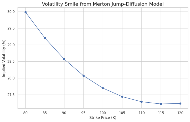
The final plot reveals the characteristic signature of a jump-diffusion model: a volatility smile. Unlike the Heston model, which with negative correlation typically produces more of a skew, the Merton model creates a good looking smile.

Why? The possibility of large jumps, both up and down, makes deep out-of-the-money options (both calls and puts) more valuable than they would be in a pure diffusion world. To justify this higher price within the Black-Scholes framework, the implied volatility must be higher for these low- and high-strike options, creating the distinct smile shape.

Kickstart your holiday campaigns

CTV should be central to any growth marketer’s Q4 strategy. And with Roku Ads Manager, launching high-performing holiday campaigns is simple and effective.

With our intuitive interface, you can set up A/B tests to dial in the most effective messages and offers, then drive direct on-screen purchases via the remote with shoppable Action Ads that integrate with your Shopify store for a seamless checkout experience.

Don’t wait to get started. Streaming on Roku picks up sharply in early October. By launching your campaign now, you can capture early shopping demand and be top of mind as the seasonal spirit kicks in.

Get a $500 ad credit when you spend your first $500 today with code: ROKUADS500. Terms apply.

Holiday performance starts now.

Conclusion: A Richer, More Realistic Toolkit

By adding a jump process to the standard diffusion model, Robert Merton provided a powerful tool for capturing a critical feature of financial markets. The jump-diffusion framework allows us to model sudden shocks, which in turn produces the fat-tailed return distributions and the volatility smiles that are consistently observed in reality.

We have now explored two major advancements over the Black-Scholes model:

• The Heston Model: Captures the continuous, mean-reverting nature of volatility, leading to realistic volatility skews.

• The Merton Model: Captures the discontinuous, sudden shocks in asset prices, leading to the classic volatility smile.

The most advanced models used in practice today, like the Bates model, actually combine both stochastic volatility and jumps to capture the best of both worlds. The journey from a simple model to these more complex frameworks is a perfect example of the quant finance ethos: start with a simple assumption. Identify where it fails to match reality. Intelligently add the necessary components to build a more robust and realistic model of the world.