
In partnership with

Take the bite out of rising vet costs with pet insurance

Veterinarians across the country have reported pressure from corporate managers to prioritize profit. This incentivized higher patient turnover, increased testing, and upselling services. Pet insurance could help you offset some of these rising costs, with some providing up to 90% reimbursement.
🚀 Your Investing Journey Just Got Better: Premium Subscriptions Are Here! 🚀
It’s been 4 months since we launched our premium subscription plans at GuruFinance Insights, and the results have been phenomenal! Now, we’re making it even better for you to take your investing game to the next level. Whether you’re just starting out or you’re a seasoned trader, our updated plans are designed to give you the tools, insights, and support you need to succeed.
Here’s what you’ll get as a premium member:
Exclusive Trading Strategies: Unlock proven methods to maximize your returns.
In-Depth Research Analysis: Stay ahead with insights from the latest market trends.
Ad-Free Experience: Focus on what matters most—your investments.
Monthly AMA Sessions: Get your questions answered by top industry experts.
Coding Tutorials: Learn how to automate your trading strategies like a pro.
Masterclasses & One-on-One Consultations: Elevate your skills with personalized guidance.
Our three tailored plans—Starter Investor, Pro Trader, and Elite Investor—are designed to fit your unique needs and goals. Whether you’re looking for foundational tools or advanced strategies, we’ve got you covered.
Don’t wait any longer to transform your investment strategy. The last 4 months have shown just how powerful these tools can be—now it’s your turn to experience the difference.

This article examines how hidden Markov models can be used to analyze historical gold price data. We discuss the mathematical framework behind hidden Markov models, illustrate the concepts with practical examples, and present a Python implementation using the pomegranate library. The goal is to uncover different market regimes that drive the changes in gold prices over time.
Introduction
Financial time series, such as gold prices, are often influenced by underlying market conditions that are not directly observable. Hidden Markov models (HMMs) offer a way to infer these latent states by assuming that the observed data are generated by an underlying stochastic process that switches between different regimes. In the context of gold prices, these regimes might represent periods of low, medium, or high volatility.
In our approach, we model the daily change in gold price rather than the raw price itself. This is because the changes can better capture the dynamics of market behavior. We assume that each regime is associated with a distinct Gaussian distribution, which reflects different volatility characteristics.
Mathematical Background
A hidden Markov model consists of two stochastic processes: one for the hidden states and one for the observations.


The hidden states evolve according to a Markov process, meaning that the probability of the current state depends only on the previous state. In mathematical terms, if the state at time t is Zₜ and the observation is Xₜ, then

Each observation Xᵢ is generated from a probability distribution that is conditioned on the hidden state. For continuous data like daily changes in gold price, it is common to assume that

Here, μᵢ and σᵢ are the mean and standard deviation associated with state i.
An HMM is fully defined by three sets of parameters:.
The initial state distribution:

The state transition probabilities:

The emission probabilities, where each state i has an associated probability density function:

The joint probability of a hidden state sequence

and an observation sequence

is given by

A Detailed Example
Imagine a simplified model with two hidden states representing “calm” and “volatile” market conditions. Let the hidden state set be

Here, state 1 indicates a calm market and state 2 indicates a volatile market. Assume that the initial probabilities are:

This suggests that the market is likely to be calm at the start.
We also assume that the transition probability matrix is:

This means that if the market is calm, it remains calm with high probability; if it is volatile, it tends to remain volatile as well.
Finally, let’s assume that the emission distributions are:

and

Thus, a day’s gold price change is modeled as a draw from one of these two distributions, depending on the current hidden state. In practice, the model would be more complex, and we might use three states to capture low, medium, and high volatility regimes.
Python Implementation with Pomegranate
The following Python code implements an HMM analysis of historical gold prices using the pomegranate’s DenseHMM and torch‐based Normal distributions. The code is organized around the GoldHMMAnalyzerclass, which encapsulates the entire workflow — from data ingestion and processing to model fitting via the Baum–Welch algorithm, hidden state decoding using the Viterbi algorithm, and result visualization.
Initially, standard libraries are imported for operating system functions, command-line interaction, data manipulation, plotting, and tensor computations. pomegranate’s Normal and DenseHMM classes are imported to construct and train the hidden Markov model.
# import required system modules
#
import os
import sys

import matplotlib as mpl
import matplotlib.pyplot as plt
import numpy as np
import pandas as pd
import torch
from pomegranate.distributions.normal import Normal
from pomegranate.hmm.dense_hmm import DenseHMM
Global parameters are defined next. In this implementation, the filename is set using its basename via os.path.basename(__file__), the number of hidden states is set to 3 (representing different market volatility regimes), the covariance type for the Gaussian emissions is set to "diag", the model is trained for a maximum of 50 iterations, and a fixed random seed (42) ensures reproducibility; additionally, matplotlib settings are configured to use LaTeX for text rendering, a serif font with a size of 12, and dashed grid lines with an alpha value of 0.5.
He’s already IPO’d once – this time’s different

Spencer Rascoff grew Zillow from seed to IPO. But everyday investors couldn’t join until then, missing early gains. So he did things differently with Pacaso. They’ve made $110M+ in gross profits disrupting a $1.3T market. And after reserving the Nasdaq ticker PCSO, you can join for $2.80/share until 5/29.
This is a paid advertisement for Pacaso’s Regulation A offering. Please read the offering circular at invest.pacaso.com. Reserving a ticker symbol is not a guarantee that the company will go public. Listing on the NASDAQ is subject to approvals. Under Regulation A+, a company has the ability to change its share price by up to 20%, without requalifying the offering with the SEC.
# set the filename using basename
#
__FILE__ = os.path.basename(__file__)

# define global constants
#
N_COMPONENTS = 3
COVARIANCE_TYPE = "diag"
N_ITER = 50
RANDOM_STATE = 42

# configure matplotlib settings
#
mpl.rcParams.update({"text.usetex": True, "font.family": "serif", "font.size": 12, "axes.grid": True, "grid.linestyle": "--", "grid.alpha": 0.5})
The GoldHMMAnalyzer class is then defined. Its constructor initializes the key parameters and reserves placeholders for the model, the decoded hidden state sequence, and the processed data.
class GoldHMMAnalyzer:
 """
 Class: GoldHMMAnalyzer

 arguments:
  none

 description:
  This class implements a Hidden Markov Model analysis for historical gold prices.
  It processes input CSV data, fits an HMM with Gaussian emissions using pomegranate’s
  DenseHMM and torch-based Normal distributions, and decodes the most likely hidden state
  sequence using the Viterbi algorithm.
 """

 def __init__(self, n_components=N_COMPONENTS, n_iter=N_ITER, random_state=RANDOM_STATE):
  """
  method: __init__

  arguments:
   n_components: Number of hidden states in the HMM.
   n_iter: Number of iterations for the Baum–Welch algorithm.
   random_state: Random seed for reproducibility.

  return:
   none

  description:
   Initializes an instance of GoldHMMAnalyzer.
  """
  self.n_components = n_components
  self.n_iter = n_iter
  self.random_state = np.random.RandomState(random_state)
  self.model = None
  self.Z = None
  self.processed_data = None
  GoldHMMAnalyzer.__CLASS_NAME__ = self.__class__.__name__
  print("%s (line: %s) %s::__init__: Instance created with n_components = %d" %
     (__FILE__, sys._getframe().f_lineno, GoldHMMAnalyzer.__CLASS_NAME__,
      self.n_components))
  #
  # end of method
The process_data method reads a CSV file containing gold price data, converts the date column to datetime objects, computes the daily gold price changes by differencing the gold price, and filters the records to include only data from January 1, 2008, onward.
 def process_data(self, filename):
  """
  method: process_data

  arguments:
   filename: String path to the CSV file containing historical gold prices.

  return:
   processed_data: A pandas DataFrame with processed gold price data.

  description:
   Loads data from the CSV file, converts the 'datetime' column to datetime objects,
   computes daily gold price changes, and filters data from 2008 onwards.
  """
  print("%s (line: %s) %s::process_data: Processing data from %s" %
     (__FILE__, sys._getframe().f_lineno, GoldHMMAnalyzer.__CLASS_NAME__,
      filename))
  data = pd.read_csv(filename)
  data["datetime"] = pd.to_datetime(data["datetime"])
  data["gold_price_change"] = data["gold_price_usd"].diff()
  self.processed_data = data[data["datetime"] >= pd.to_datetime("2008-01-01")]
  self.processed_data = self.processed_data.dropna(subset=["gold_price_change"])
  return self.processed_data
  #
  # end of method
Once the data is processed, the compute_result method converts the series of gold price changes into a torch tensor with the appropriate shape, initializes an HMM composed of uninitialized Normal distributions, fits the model using the Baum–Welch algorithm, and decodes the most likely hidden state sequence using the Viterbi algorithm.
 def compute_result(self, processed_data):
  """
  method: compute_result

  arguments:
   processed_data: A DataFrame returned by process_data.

  return:
   result: A tuple containing (fitted HMM model, predicted hidden states).

  description:
   Converts the gold price change series to a torch tensor, initializes an HMM with
   uninitialized Normal distributions, fits the HMM using the Baum–Welch algorithm,
   and decodes the most likely hidden state sequence using the Viterbi algorithm.
  """
  print("%s (line: %s) %s::compute_result: Computing result" %
     (__FILE__, sys._getframe().f_lineno, GoldHMMAnalyzer.__CLASS_NAME__))
  X_seq = processed_data["gold_price_change"].values.astype(np.float32)
  X_tensor = torch.tensor(X_seq).unsqueeze(0).unsqueeze(-1)
  distributions = [Normal(covariance_type=COVARIANCE_TYPE) for _ in range(self.n_components)]
  model = DenseHMM(distributions=distributions, init="random", max_iter=self.n_iter,
                    random_state=self.random_state, verbose=True)
  model.fit(X_tensor)
  Z = model.viterbi(X_tensor)
  self.model = model
  self.Z = Z[0].detach().numpy()
  return (self.model, self.Z)
  #
  # end of method
Finally, the format_output method gathers and formats the key model parameters, including the unique hidden states, the starting probabilities, the state transition matrix (with log probabilities converted to probability space), and the Gaussian parameters (means and covariances) for each state.
 def format_output(self, result):
  """
  method: format_output

  arguments:
   result: A tuple containing (model, hidden states).

  return:
   output: A formatted string representation of the HMM parameters.

  description:
   Extracts and formats the HMM parameters including unique states, start probabilities,
   transition matrix, Gaussian means, and Gaussian covariances.
   The stored probabilities are in log-space and are converted to probability space.
  """
  print("%s (line: %s) %s::format_output: Formatting output" %
     (__FILE__, sys._getframe().f_lineno, GoldHMMAnalyzer.__CLASS_NAME__))
  model, Z = result
  start_probs = torch.exp(model.starts).detach().cpu().numpy() if model.starts is not None else None
  transmat = torch.exp(model.edges).detach().cpu().numpy() if model.edges is not None else None
  means = []
  covars = []
  for dist in model.distributions:
   means.append(dist.means.detach().cpu().numpy())
   covars.append(dist.covs.detach().cpu().numpy())
  means = np.array(means)
  covars = np.array(covars)
  output = []
  output.append("\nUnique states:\n{}".format(np.unique(Z)))
  output.append("\nStart probabilities:\n{}".format(start_probs))
  output.append("\nTransition matrix:\n{}".format(transmat))
  output.append("\nGaussian means:\n{}".format(means))
  output.append("\nGaussian covariances:\n{}\n".format(covars))
  return "\n".join(output)
  #
  # end of method
The main routine ties together the complete workflow. It verifies the input file provided via the command line, processes the gold price data, fits the HMM and decodes the hidden states, prints the formatted model parameters, and generates two plots. The first plot displays the historical gold prices over time with data points color-coded by the inferred hidden states, while the second plot shows the daily gold price changes similarly annotated, thereby highlighting periods of distinct market volatility.
def main():
 """
 method: main

 arguments:
  none (input is expected via command line arguments)

 return:
  none

 description:
  Main routine to execute the gold price analysis.
  Reads input data from a CSV file, processes the data, computes results by fitting
  an HMM and decoding hidden states, and generates plots to visualize the gold price
  and price change data with the inferred hidden states.
 """
 if len(sys.argv) < 2:
  print("Usage: {} <input_file>".format(sys.argv[0]))
  sys.exit(1)

 filename = sys.argv[1]

 print("%s (line: %s) %s::%s: Reading input file: %s" %
    (__FILE__, sys._getframe().f_lineno, "main", "__init__", filename))

 algorithm = GoldHMMAnalyzer()

 processed_data = algorithm.process_data(filename)

 result = algorithm.compute_result(processed_data)

 output = algorithm.format_output(result)

 print("%s (line: %s) %s::%s: Output: %s" %
    (__FILE__, sys._getframe().f_lineno, "main", "__init__", output))

 print("%s (line: %s) %s::%s: Generating plots" %
    (__FILE__, sys._getframe().f_lineno, "main", "__init__"))
 fig, axs = plt.subplots(2, 1, figsize=(15, 10), dpi=300, sharex=True)
 unique_states = np.unique(algorithm.Z)

 for state in unique_states:
  mask = (algorithm.Z == state)
  axs[0].plot(
   processed_data["datetime"].iloc[mask],
   processed_data["gold_price_usd"].iloc[mask],
   marker="o", linestyle="none", label=f"State {state}"
  )
 axs[0].set_title(r"\textbf{Gold Price Over Time by Hidden State}")
 axs[0].set_ylabel(r"\textbf{Gold Price (USD)}")
 axs[0].legend(title="Hidden States", title_fontsize="large")
 axs[0].grid(True)

 for state in unique_states:
  mask = (algorithm.Z == state)
  axs[1].plot(
   processed_data["datetime"].iloc[mask],
   processed_data["gold_price_change"].iloc[mask],
   marker="o", linestyle="none", label=f"State {state}"
  )
 axs[1].set_title(r"\textbf{Gold Price Change Over Time by Hidden State}")
 axs[1].set_xlabel(r"\textbf{Date}")
 axs[1].set_ylabel(r"\textbf{Gold Price Change (USD)}")
 axs[1].legend(title="Hidden States", title_fontsize="large")
 axs[1].grid(True)

 plt.tight_layout()
 plt.show()
 #
 # end of method
Running the script on a historical gold price dataset prints detailed model parameters to the console. In particular, you will observe the unique hidden states, the starting probabilities, the state-to-state transition matrix, and the Gaussian parameters (means and covariances) for each state. These numerical outputs provide a quantitative description of the regimes that drive the observed price changes.
p01.py (line: 226) main::__init__: Output:
Unique states:
[0 1 2]

Start probabilities:
[3.0482917e-24 1.0000000e+00 0.0000000e+00]

Transition matrix:
[[6.5476710e-01 3.2066992e-01 2.4534980e-02]
 [2.1438229e-01 7.8494406e-01 1.6365851e-04]
 [7.9335861e-02 2.0831732e-04 9.2044955e-01]]

Gaussian means:
[[0.20836642]
 [0.24445221]
 [0.4723044 ]]

Gaussian covariances:
[[144.2576  ]
 [ 30.039436]
 [491.6002  ]]
In addition, two informative plots are generated. The first plot displays the gold price time series over time, with each data point color-coded according to its inferred hidden state, thereby revealing shifts between different market regimes. The second plot illustrates the daily gold price changes with the hidden states overlaid, highlighting periods of varying volatility.
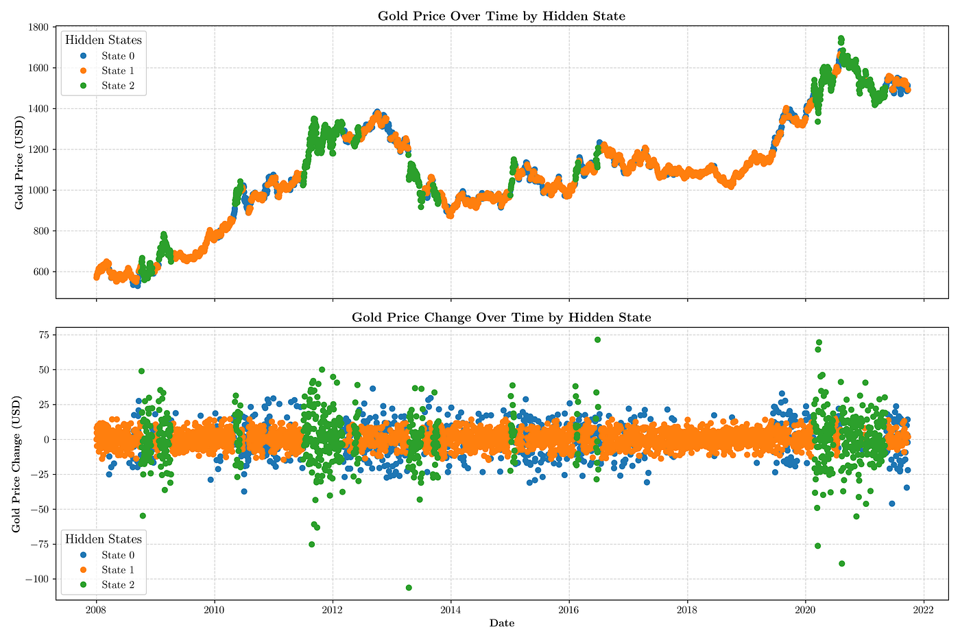
Hidden Markov Model Analysis of Historical Gold Prices — The upper plot displays the gold price time series annotated by the inferred hidden states, and the lower plot illustrates the corresponding daily price changes with state annotations, offering insights into different market volatility regimes.
Conclusion
This work demonstrates how hidden Markov models can be effectively applied to analyze financial time series data, such as historical gold prices. By modeling the daily price changes as originating from a process that alternates between different volatility regimes, we obtain insights into the underlying market dynamics. The pomegranate library in Python simplifies the implementation of these models, allowing for parameter estimation via the Baum-Welch algorithm and state inference through the Viterbi method.
The detailed model parameters and visualizations provide a clear picture of the latent structure in the gold price data. This framework can serve as a basis for further research, including real-time regime detection or extension to other financial instruments.