The Supply Chain Crisis Is Escalating — But This Tech Startup Keeps Winning

Global supply chain chaos is intensifying. Major retailers warn of holiday shortages, and tech giants are slashing forecasts as parts dry up.

But while others scramble, one smart home innovator is thriving.

Their strategic move to manufacturing outside China has kept production running smoothly — driving 200% year-over-year growth, even as the industry stalls.

This foresight is no accident. The same leadership team that saw the supply chain storm coming has already expanded into over 120 BestBuy locations, with talks underway to add Walmart and Home Depot.

At just $1.90 per share, this resilient tech startup offers rare stability in uncertain times. As investors flee vulnerable companies, this window is closing fast.

SECURE YOUR POSITION BEFORE PRICES RISE

_{Past performance is not indicative of future results. Email may contain forward-looking statements. See US Offering for details. Informational purposes only.}

🚀 Your Investing Journey Just Got Better: Premium Subscriptions Are Here! 🚀

It’s been 4 months since we launched our premium subscription plans at GuruFinance Insights, and the results have been phenomenal! Now, we’re making it even better for you to take your investing game to the next level. Whether you’re just starting out or you’re a seasoned trader, our updated plans are designed to give you the tools, insights, and support you need to succeed.

Here’s what you’ll get as a premium member:

• Exclusive Trading Strategies: Unlock proven methods to maximize your returns.

• In-Depth Research Analysis: Stay ahead with insights from the latest market trends.

• Ad-Free Experience: Focus on what matters most—your investments.

• Monthly AMA Sessions: Get your questions answered by top industry experts.

• Coding Tutorials: Learn how to automate your trading strategies like a pro.

• Masterclasses & One-on-One Consultations: Elevate your skills with personalized guidance.

Our three tailored plans—Starter Investor, Pro Trader, and Elite Investor—are designed to fit your unique needs and goals. Whether you’re looking for foundational tools or advanced strategies, we’ve got you covered.

Don’t wait any longer to transform your investment strategy. The last 4 months have shown just how powerful these tools can be—now it’s your turn to experience the difference.

👉 Explore Premium Plans Now

The Power of Adaptive Leverage in Trading

Many traders face a dilemma: shorting individual stocks carries substantial risks from unexpected news, earnings surprises, and volatility spikes. Yet a strict long-only approach may sacrifice potential returns during market downturns.

What if we could enhance a long-only strategy with tactical leverage?

The Multi-Regime Adaptive Leverage Strategy (MRALS) offers precisely this solution: applying varying levels of leverage (0x to 3x) based on market conditions while maintaining a long-only discipline.

Smarter Investing Starts with Smarter News

The Daily Upside helps 1M+ investors cut through the noise with expert insights. Get clear, concise, actually useful financial news. Smarter investing starts in your inbox—subscribe free.

Join 1M+ readers today.

MRALS Strategy Overview

MRALS combines three key innovations:

1. Adaptive leverage based on market regimes: Applying 0–3x leverage depending on volatility conditions.

2. Yang-Zhang volatility measurement: Using superior volatility detection that captures overnight gaps.

3. Realistic trade execution: Generating signals at market close but executing at the next day’s open.

Rather than attempting to short during downturns, MRALS shifts to cash (0x exposure) in high-volatility environments while amplifying exposure (up to 3x) during favorable conditions.

Strategy Components

The strategy classifies market conditions into four distinct regimes:

• Aggressive (3x leverage): Low volatility + strong bullish trend + normal VIX term structure.

• Bullish (2x leverage): Positive trend with moderate volatility.

• Moderate (1x leverage): Neutral conditions.

• Defensive (0x leverage): High volatility or bearish signals.

A hybrid oscillator combining price momentum and volatility metrics generates entry and exit signals, while the Yang-Zhang volatility model provides more accurate risk assessment than traditional methods.

import pandas as pd
import numpy as np
import yfinance as yf
import matplotlib.pyplot as plt
from matplotlib.gridspec import GridSpec

def fetch_data(ticker, start_date, end_date=None):
    """Downloads data including OHLC and the actual VIX and VIX3M indices"""
    # Data download
    data = yf.download(ticker, start=start_date, end=end_date)
    vix = yf.download("^VIX", start=start_date, end=end_date)['Close']
    vix3m = yf.download("^VIX3M", start=start_date, end=end_date)['Close']
    
    df = pd.DataFrame(index=data.index)
    df['Open'] = data['Open']
    df['High'] = data['High'] 
    df['Low'] = data['Low']
    df['Close'] = data['Close']
    df['Volume'] = data['Volume']
    df['VIX'] = vix
    df['VIX3M'] = vix3m  # Use the actual VIX3M instead of the synthetic version
    df['VIX_Ratio'] = df['VIX'] / df['VIX3M']
    
    return df.dropna()

def calculate_yang_zhang_volatility(data, window=21):
    """Calculates Yang-Zhang volatility"""
    open_price = data['Open']
    high_price = data['High']
    low_price = data['Low']
    close_price = data['Close']
    
    # Logarithmic calculations
    log_ho = np.log(high_price / open_price)
    log_lo = np.log(low_price / open_price)
    log_oc = np.log(close_price / open_price)
    log_co = np.log(open_price / close_price.shift(1))
    
    # Volatility components
    rs = log_ho * (log_ho - log_oc) + log_lo * (log_lo - log_oc)
    close_vol = log_oc**2
    open_vol = log_co**2
    
    # Moving values
    rs_roll = rs.rolling(window=window).mean()
    close_roll = close_vol.rolling(window=window).mean()
    open_roll = open_vol.rolling(window=window).mean()
    
    # Optimal k factor for Yang-Zhang
    k = 0.34 / (1.34 + (window + 1) / (window - 1))
    
    # YZ Volatility
    yz_vol = np.sqrt(open_roll + k * close_roll + (1 - k) * rs_roll)
    
    # Annualize (multiply by sqrt(252))
    return yz_vol * np.sqrt(252)

def calculate_oscillator(data):
    """Creates a hybrid oscillator"""
    # Momentum component (differential EMA)
    ema_fast = data['Close'].ewm(span=8, adjust=False).mean()
    ema_slow = data['Close'].ewm(span=21, adjust=False).mean()
    
    momentum = ((ema_fast / ema_slow) - 1) * 100
    
    # Relative strength component
    rel_strength = data['Close'].pct_change(21) - data['Close'].pct_change(21).rolling(252).mean()
    rel_strength = rel_strength / rel_strength.rolling(63).std().fillna(0.0001)
    
    # Volatility component
    vol_ratio = data['VIX_Ratio'] - data['VIX_Ratio'].rolling(21).mean()
    vol_ratio = vol_ratio / vol_ratio.rolling(63).std().fillna(0.0001)
    
    # Final oscillator (weighted combination)
    oscillator = (0.5 * momentum) + (0.3 * rel_strength) - (0.2 * vol_ratio)
    
    # Smoothing to reduce noise
    oscillator_smooth = oscillator.ewm(span=5, adjust=False).mean()
    
    return oscillator_smooth

def detect_market_regime(data, yz_vol, oscillator):
    """Detects the market regime and determines the leverage factor"""
    # Classify volatility
    vol_percentile = yz_vol.rolling(252).rank(pct=True).fillna(0.5)
    low_vol = vol_percentile < 0.2
    high_vol = vol_percentile > 0.8
    
    # Price trend
    price_trend = data['Close'] > data['Close'].rolling(50).mean()
    price_momentum = data['Close'].pct_change(63) > 0
    
    # VIX indicator
    vix_contango = data['VIX_Ratio'] < 0.9  # VIX < VIX3M (normal market)
    vix_backwardation = data['VIX_Ratio'] > 1.1  # VIX > VIX3M (market stress)
    
    # Oscillator signal
    oscillator_bullish = oscillator > 0.5
    oscillator_bearish = oscillator < -0.5
    
    # Determine regime
    regime = pd.Series(index=data.index, dtype='object')
    
    # Condition combinations
    regime[oscillator_bullish & low_vol & price_trend & vix_contango] = 'Aggressive'  # 3x
    regime[oscillator_bullish & price_trend & ~high_vol] = 'Bullish'  # 2x
    regime[(~oscillator_bearish & ~oscillator_bullish) | 
           (price_momentum & ~high_vol)] = 'Moderate'  # 1x
    regime[oscillator_bearish | high_vol | vix_backwardation] = 'Defensive'  # 0x
    
    # Fill NA values with 'Moderate'
    regime = regime.fillna('Moderate')
    
    # Convert to leverage factor
    leverage_factor = pd.Series(index=data.index)
    leverage_factor[regime == 'Aggressive'] = 3.0
    leverage_factor[regime == 'Bullish'] = 2.0
    leverage_factor[regime == 'Moderate'] = 1.0
    leverage_factor[regime == 'Defensive'] = 0.0
    
    return regime, leverage_factor

def generate_signals(data, oscillator, leverage_factor):
    """Generates signals based on the oscillator and market regime"""
    signals = pd.DataFrame(index=data.index)
    signals['Close'] = data['Close']
    signals['Open'] = data['Open']
    signals['Oscillator'] = oscillator
    signals['Regime'] = leverage_factor
    
    # Initialize columns
    signals['Signal'] = 0
    signals['Entry'] = 0
    signals['Exit'] = 0
    signals['Position'] = 0
    signals['Leverage'] = 0
    
    # Moving average of the oscillator for crossover
    oscillator_ma = oscillator.rolling(window=13).mean()
    
    # Generate signals
    for i in range(13, len(signals)):
        # Current and previous values
        curr_osc = oscillator.iloc[i]
        prev_osc = oscillator.iloc[i-1]
        curr_ma = oscillator_ma.iloc[i]
        prev_ma = oscillator_ma.iloc[i-1]
        curr_lev = leverage_factor.iloc[i]
        
        # Entry signal: crossover or regime improvement
        if ((prev_osc <= prev_ma and curr_osc > curr_ma) or 
            (signals['Position'].iloc[i-1] == 0 and curr_lev >= 1.0 and 
             signals['Leverage'].iloc[i-1] < 1.0)):
            signals.loc[signals.index[i], 'Signal'] = 1
            signals.loc[signals.index[i], 'Entry'] = 1
        
        # Exit signal: crossunder or defensive regime
        elif ((prev_osc >= prev_ma and curr_osc < curr_ma) or 
              (signals['Position'].iloc[i-1] > 0 and curr_lev == 0)):
            signals.loc[signals.index[i], 'Signal'] = -1
            signals.loc[signals.index[i], 'Exit'] = 1
        
        # Position adjustment if leverage changes without exiting
        elif (signals['Position'].iloc[i-1] > 0 and 
              curr_lev != signals['Leverage'].iloc[i-1] and 
              curr_lev > 0):
            signals.loc[signals.index[i], 'Signal'] = 2  # Adjustment signal
        
        # Calculate position and leverage
        if signals['Entry'].iloc[i] == 1:
            signals.loc[signals.index[i], 'Position'] = 1
            signals.loc[signals.index[i], 'Leverage'] = curr_lev
        elif signals['Exit'].iloc[i] == 1:
            signals.loc[signals.index[i], 'Position'] = 0
            signals.loc[signals.index[i], 'Leverage'] = 0
        elif signals['Signal'].iloc[i] == 2:  # Adjustment
            signals.loc[signals.index[i], 'Position'] = 1
            signals.loc[signals.index[i], 'Leverage'] = curr_lev
        else:
            signals.loc[signals.index[i], 'Position'] = signals['Position'].iloc[i-1]
            signals.loc[signals.index[i], 'Leverage'] = signals['Leverage'].iloc[i-1]
    
    return signals

def backtest_strategy(signals, initial_capital=100000):
    """Executes backtest with entry at the next day's open"""
    backtest = signals.copy()
    
    # Prepare for backtesting with entry on the next day
    backtest['Next_Open'] = backtest['Open'].shift(-1)
    
    # Initialize backtest columns
    backtest['Trade_Entry'] = np.nan
    backtest['Trade_Exit'] = np.nan
    backtest['Trade_Return'] = np.nan
    backtest['Strategy_Return'] = 0.0
    
    # Trade tracking
    in_position = False
    entry_price = 0
    entry_date = None
    entry_leverage = 0
    
    # Process day by day
    for i in range(len(backtest)-1):  # Ignore last day
        current_date = backtest.index[i]
        next_date = backtest.index[i+1]
        
        # Buy signal at close = entry next day
        if backtest['Entry'].iloc[i] == 1 and not in_position:
            entry_price = backtest['Next_Open'].iloc[i]
            entry_date = next_date
            entry_leverage = backtest['Leverage'].iloc[i]
            in_position = True
            
            backtest.loc[next_date, 'Trade_Entry'] = entry_price
            
        # Sell signal at close = exit next day
        elif backtest['Exit'].iloc[i] == 1 and in_position:
            exit_price = backtest['Next_Open'].iloc[i]
            
            # Calculate trade return
            trade_return = (exit_price / entry_price - 1) * entry_leverage
            
            # Record exit
            backtest.loc[next_date, 'Trade_Exit'] = exit_price
            backtest.loc[next_date, 'Trade_Return'] = trade_return
            
            # Reset
            in_position = False
            entry_price = 0
            entry_date = None
            entry_leverage = 0
            
        # Leverage adjustment (without closing position)
        elif backtest['Signal'].iloc[i] == 2 and in_position:
            new_leverage = backtest['Leverage'].iloc[i]
            entry_leverage = new_leverage
    
    # Calculate daily strategy returns
    for i in range(1, len(backtest)-1):
        if backtest['Position'].iloc[i] == 1:
            # Return from current open to next open
            daily_return = backtest['Next_Open'].iloc[i] / backtest['Open'].iloc[i] - 1
            leveraged_return = daily_return * backtest['Leverage'].iloc[i]
            backtest.loc[backtest.index[i+1], 'Strategy_Return'] = leveraged_return
    
    # Calculate equity curve
    backtest['Strategy_Equity'] = (1 + backtest['Strategy_Return'].fillna(0)).cumprod()
    
    # Buy & hold for comparison
    backtest['BuyHold_Return'] = backtest['Open'].pct_change()
    backtest['BuyHold_Equity'] = (1 + backtest['BuyHold_Return'].fillna(0)).cumprod()
    
    # Drawdowns
    backtest['Strategy_Peak'] = backtest['Strategy_Equity'].expanding().max()
    backtest['Strategy_Drawdown'] = backtest['Strategy_Equity'] / backtest['Strategy_Peak'] - 1
    
    backtest['BuyHold_Peak'] = backtest['BuyHold_Equity'].expanding().max()
    backtest['BuyHold_Drawdown'] = backtest['BuyHold_Equity'] / backtest['BuyHold_Peak'] - 1
    
    return backtest

def calculate_metrics(backtest):
    """Calculates performance metrics"""
    # Filter returns
    strategy_returns = backtest['Strategy_Return'].dropna()
    bh_returns = backtest['BuyHold_Return'].dropna()
    trade_returns = backtest['Trade_Return'].dropna()
    
    if len(strategy_returns) == 0:
        return {
            'Total Return': 0,
            'Annual Return': 0,
            'Annual Volatility': 0,
            'Sharpe Ratio': 0,
            'Max Drawdown': 0,
            'Number of Trades': 0,
            'Win Rate': 0,
            'Average Win': 0,
            'Average Loss': 0,
            'Time in Market': 0,
            'Average Exposure': 0,
            'BH Total Return': 0,
            'BH Annual Return': 0,
            'BH Annual Volatility': 0,
            'BH Sharpe Ratio': 0,
            'BH Max Drawdown': 0
        }
    
    # Calculate metrics
    metrics = {}
    
    # Total and annual
    metrics['Total Return'] = backtest['Strategy_Equity'].iloc[-1] - 1
    years = len(backtest) / 252
    metrics['Annual Return'] = (1 + metrics['Total Return']) ** (1/years) - 1
    
    # Risk
    metrics['Annual Volatility'] = strategy_returns.std() * np.sqrt(252)
    metrics['Sharpe Ratio'] = metrics['Annual Return'] / metrics['Annual Volatility'] if metrics['Annual Volatility'] > 0 else 0
    metrics['Max Drawdown'] = backtest['Strategy_Drawdown'].min()
    
    # Trade statistics
    metrics['Number of Trades'] = len(trade_returns)
    metrics['Win Rate'] = (trade_returns > 0).mean() if len(trade_returns) > 0 else 0
    metrics['Average Win'] = trade_returns[trade_returns > 0].mean() if len(trade_returns[trade_returns > 0]) > 0 else 0
    metrics['Average Loss'] = trade_returns[trade_returns < 0].mean() if len(trade_returns[trade_returns < 0]) > 0 else 0
    
    # Time in market
    metrics['Time in Market'] = (backtest['Position'] > 0).mean()
    
    # Average exposure (considering leverage)
    metrics['Average Exposure'] = backtest['Leverage'].mean()
    
    # Buy & Hold
    metrics['BH Total Return'] = backtest['BuyHold_Equity'].iloc[-1] - 1
    metrics['BH Annual Return'] = (1 + metrics['BH Total Return']) ** (1/years) - 1
    metrics['BH Annual Volatility'] = bh_returns.std() * np.sqrt(252)
    metrics['BH Sharpe Ratio'] = metrics['BH Annual Return'] / metrics['BH Annual Volatility'] if metrics['BH Annual Volatility'] > 0 else 0
    metrics['BH Max Drawdown'] = backtest['BuyHold_Drawdown'].min()
    
    return metrics

def plot_results(backtest, yz_vol, oscillator, regime, metrics):
    """Visualizes the strategy results"""
    # Configuration
    fig = plt.figure(figsize=(15, 18))
    gs = GridSpec(4, 2, height_ratios=[2, 1, 1, 1], hspace=0.4, wspace=0.3)
    
    # 1. Price and signals
    ax1 = fig.add_subplot(gs[0, :])
    ax1.plot(backtest.index, backtest['Close'], color='blue', label='Price', alpha=0.7)
    
    # Mark entries and exits
    entries = backtest.dropna(subset=['Trade_Entry'])
    exits = backtest.dropna(subset=['Trade_Exit'])
    
    # Differentiate entries by leverage
    if len(entries) > 0:
        for i, row in entries.iterrows():
            marker_size = 50 + 50 * row['Leverage']  # Size based on leverage
            ax1.scatter(i, row['Trade_Entry'], color='green', marker='^', 
                      s=marker_size, alpha=0.7)
    
    if len(exits) > 0:
        ax1.scatter(exits.index, exits['Trade_Exit'], color='red', marker='v', 
                  s=100, alpha=0.7, label='Exit')
    
    ax1.set_title('Price with Trading Signals', fontsize=14)
    ax1.set_ylabel('Price', fontsize=12)
    ax1.legend(loc='upper left')
    ax1.grid(True, alpha=0.3)
    
    # 2. Oscillator
    ax2 = fig.add_subplot(gs[1, 0:1])
    ax2.plot(backtest.index, oscillator, label='Oscillator', color='purple')
    ax2.plot(backtest.index, oscillator.rolling(13).mean(), label='MA(13)', 
            color='orange', linestyle='--')
    ax2.axhline(y=0, color='black', linestyle='-', alpha=0.3)
    
    ax2.set_title('Hybrid Oscillator', fontsize=14)
    ax2.set_ylabel('Value', fontsize=12)
    ax2.legend()
    ax2.grid(True, alpha=0.3)
    
    # 3. Yang-Zhang Volatility
    ax3 = fig.add_subplot(gs[1, 1:2])
    ax3.plot(backtest.index, yz_vol, label='YZ Volatility', color='red')
    
    ax3.set_title('Yang-Zhang Annualized Volatility', fontsize=14)
    ax3.set_ylabel('Volatility', fontsize=12)
    ax3.legend()
    ax3.grid(True, alpha=0.3)
    
    # 4. Exposure / Leverage
    ax4 = fig.add_subplot(gs[2, :])
    ax4.plot(backtest.index, backtest['Leverage'], label='Leverage Factor',
            color='orange', linewidth=2)
    ax4.set_title('Exposure / Leverage', fontsize=14)
    ax4.set_ylabel('Factor (x)', fontsize=12)
    ax4.set_ylim(0, 3.5)
    ax4.legend()
    ax4.grid(True, alpha=0.3)
    
    # 5. Equity Curves
    ax5 = fig.add_subplot(gs[3, :])
    ax5.plot(backtest.index, backtest['Strategy_Equity'], label='MRALS Strategy', 
            color='blue', linewidth=2)
    ax5.plot(backtest.index, backtest['BuyHold_Equity'], label='Buy & Hold', 
            color='gray', linestyle='--', alpha=0.7)
    
    ax5.set_title('Equity Curves', fontsize=14)
    ax5.set_ylabel('Equity (Normalized)', fontsize=12)
    ax5.set_xlabel('Date', fontsize=12)
    ax5.legend()
    ax5.grid(True, alpha=0.3)
    
    # Add metrics table
    metrics_text = (
        f"MRALS STRATEGY vs BUY & HOLD\n"
        f"='='='='='='='='='='='='='='\n"
        f"Total Return: {metrics['Total Return']*100:.2f}% vs {metrics['BH Total Return']*100:.2f}%\n"
        f"Annual Return: {metrics['Annual Return']*100:.2f}% vs {metrics['BH Annual Return']*100:.2f}%\n"
        f"Volatility: {metrics['Annual Volatility']*100:.2f}% vs {metrics['BH Annual Volatility']*100:.2f}%\n"
        f"Sharpe Ratio: {metrics['Sharpe Ratio']:.2f} vs {metrics['BH Sharpe Ratio']:.2f}\n"
        f"Maximum Drawdown: {metrics['Max Drawdown']*100:.2f}% vs {metrics['BH Max Drawdown']*100:.2f}%\n\n"
        f"ADDITIONAL STATISTICS\n"
        f"='='='='='='='='='='='='='\n"
        f"Number of Trades: {int(metrics['Number of Trades'])}\n"
        f"Win Rate: {metrics['Win Rate']*100:.2f}%\n"
        f"Average Win: {metrics['Average Win']*100:.2f}%\n"
        f"Average Loss: {metrics['Average Loss']*100:.2f}%\n"
        f"Time in Market: {metrics['Time in Market']*100:.2f}%\n"
        f"Average Exposure: {metrics['Average Exposure']:.2f}x"
    )
    
    # Add text box with metrics
    props = dict(boxstyle='round', facecolor='wheat', alpha=0.4)
    ax5.text(0.02, 0.02, metrics_text, transform=ax5.transAxes, fontsize=10,
            verticalalignment='bottom', horizontalalignment='left', bbox=props)
    
    plt.tight_layout()
    plt.show()

def run_strategy(ticker='SPY', start_date='2015-01-01', end_date=None):
    """Executes the complete strategy"""
    # Download data
    data = fetch_data(ticker, start_date, end_date)
    
    # Calculate Yang-Zhang volatility
    yz_vol = calculate_yang_zhang_volatility(data)
    
    # Calculate hybrid oscillator
    oscillator = calculate_oscillator(data)
    
    # Detect market regime and leverage factor
    regime, leverage_factor = detect_market_regime(data, yz_vol, oscillator)
    
    # Generate signals
    signals = generate_signals(data, oscillator, leverage_factor)
    
    # Execute backtest
    backtest = backtest_strategy(signals)
    
    # Calculate metrics
    metrics = calculate_metrics(backtest)
    
    # Visualize results
    plot_results(backtest, yz_vol, oscillator, regime, metrics)
    
    return backtest, metrics

# Example usage
backtest, metrics = run_strategy('SPY', '2018-01-01')

Risk Management Focus

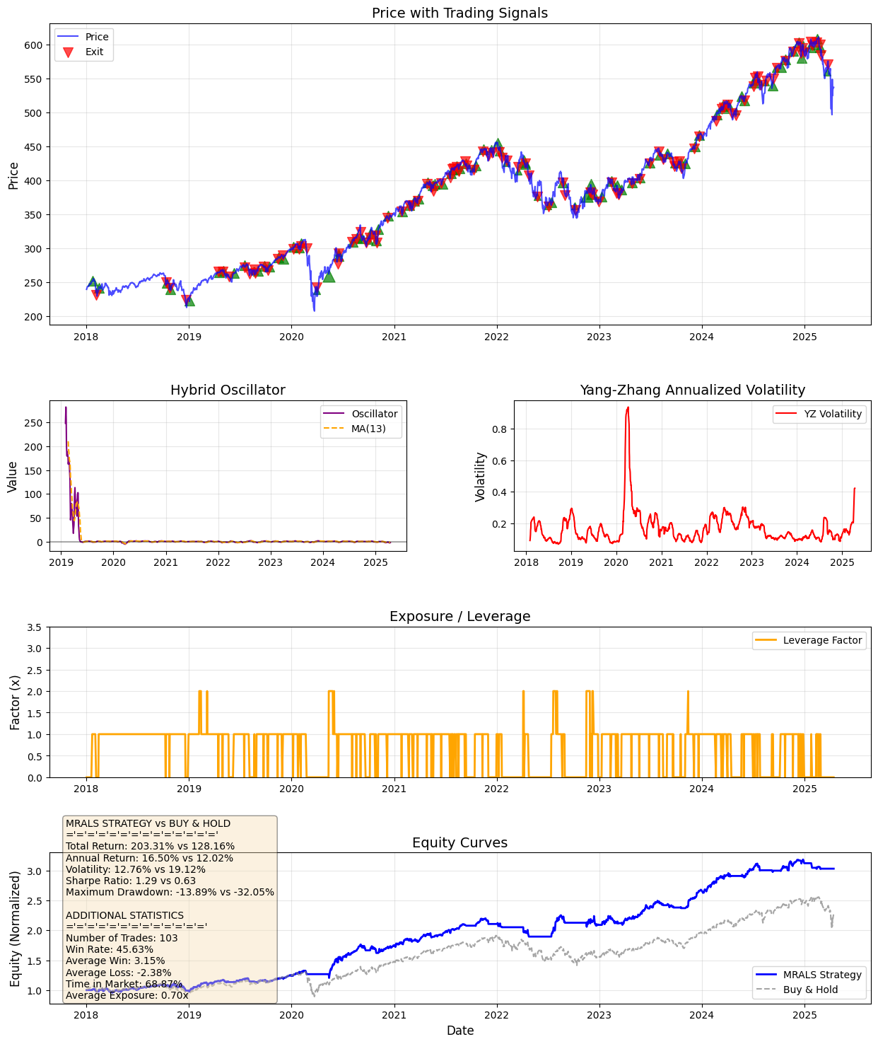
The strategy completed 103 trades with a 45.63% win rate. While this may appear modest, the average winning trade (+3.15%) exceeded the average losing trade (-2.38%), creating positive expectancy.

Most importantly, MRALS spent only 68.67% of time in the market, moving to cash during unfavorable conditions. The average leverage of 0.70x, below the neutral 1.0x position, demonstrates the strategy’s conservative approach to risk management.

Conclusion

MRALS demonstrates that a long-only approach can be significantly enhanced through tactical leverage without resorting to shorting. By applying greater exposure during favorable conditions and stepping aside during turbulent periods, the strategy achieved 59% higher returns than buy & hold while dramatically reducing volatility and drawdowns.

The combination of Yang-Zhang volatility measurement and adaptive leverage provides a compelling framework for investors who want to remain long-only but seek enhanced returns beyond traditional buy-and-hold approaches.