Invest Wisely with The Daily Upside

In this current market landscape, we all face a common challenge.

Many conventional financial news sources are driven by the pursuit of maximum clicks. Consequently, they resort to disingenuous headlines and fear-based tactics to meet their bottom line.

Luckily, we have The Daily Upside. Created by Wall Street insiders and bankers, this fresh, insightful newsletter delivers valuable market insights that go beyond the headlines. And the best part? It’s completely free.

Join 1M+ readers and subscribe today.

Exciting News: Paid Subscriptions Have Launched! 🚀

On September 1, we officially rolled out our new paid subscription plans at GuruFinance Insights, offering you the chance to take your investing journey to the next level! Whether you're just starting or are a seasoned trader, these plans are packed with exclusive trading strategies, in-depth research paper analysis, ad-free content, monthly AMAsessions, coding tutorials for automating trading strategies, and much more.

Our three tailored plans—Starter Investor, Pro Trader, and Elite Investor—provide a range of valuable tools and personalized support to suit different needs and goals. Don’t miss this opportunity to get real-time trade alerts, access to masterclasses, one-on-one strategy consultations, and be part of our private community group. Click here to explore the plans and see how becoming a premium member can elevate your investment strategy!

In the financial markets, where a lot of money can be gained or lost within seconds, traders are always searching for some element of risk and return balance in their strategies. One of these strategies is the pair trading. This strategy is market neutral, hence traders do not expect any absolute price movements in the instruments involved but only the price differential between the two correlated instruments.

In this article, we will be looking at how pair trading can be applied in the example of two leaders in technology: Apple (AAPL) and Microsoft (MSFT). You will also learn how to implement one such statistical arbitrage strategy outlining the steps of cointegration analysis, hedge ratio determination, and spread development. Finally, we will illustrate how to carry out a backtest on the strategy and evaluate its results based on factors, including but not limited to, returns, volatility, the Sharpe Ratio, and the maximal drawdown.

In the end, you will get to learn the basic processes involved in pair trading and also how such a strategy could be geared to work perfectly in real market situations.

Borrow up to $800 to cover unexpected expenses!

Spotloan is a better way to borrow extra money when you need it. It’s not a payday loan. It’s an installment loan, which means you pay down the balance with each on-time payment. Borrow up to $1,500 (up to $800 for new and repeat borrowers, up to $1,500 for preferred customers with 10 or more loans). Then, pay Spotloan back a little at a time.

Spotloan let's you get money fast. Most people complete the application and find out if they're approved within minutes! Plus Spotloan can offer loans at up to half the cost other small-dollar lenders, payday companies, and pawn brokers... without the hidden fees!

Spotloan can help with all of life's emergency expenses, from hospital bills to car emergencies to a sick pet or a broken cell phone.

Learn More

1. Importing Libraries and Data

To start, we need to import several Python libraries that will help us analyze the data and run our pair trading strategy.

import pandas as pd
import numpy as np
import yfinance as yf
from sklearn.linear_model import LinearRegression
from statsmodels.tsa.stattools import coint
import matplotlib.pyplot as plt
import seaborn as sns

These libraries are essential for handling data, running statistical tests, and plotting results. Yahoo Finance (yfinance) provides the historical stock data for Apple and Microsoft. Pandas helps in data manipulation, while NumPy supports numerical computations. Accessing clean, historical data is the foundation of any successful trading strategy. It allows us to examine price movements, perform tests, and backtest strategies accurately.

2. Downloading Price Data for AAPL and MSFT

Now, we will download the historical data for Apple (AAPL) and Microsoft (MSFT) from January 2015 to October 2023.

ticker1 = 'AAPL'
ticker2 = 'MSFT'
start_date = '2015-01-01'
end_date = '2023-10-01'
data1 = yf.download(ticker1, start=start_date, end=end_date)
data2 = yf.download(ticker2, start=start_date, end=end_date)

This code fetches the adjusted closing prices for both companies. The adjusted close price is important as it reflects all corporate actions like dividends and stock splits, giving a true representation of the stock’s value.

Having accurate and adjusted price data ensures that we are basing our analysis on realistic, market-reflective values. This is crucial when analyzing long-term trends and making predictions about future movements.

3. Visualizing Price Series

We can now visualize how the prices of Apple and Microsoft have moved over time.

plt.figure(figsize=(14, 7))
plt.plot(df[ticker1], label=ticker1)
plt.plot(df[ticker2], label=ticker2)
plt.title('Price Series of AAPL and MSFT')
plt.xlabel('Date')
plt.ylabel('Adjusted Close Price')
plt.legend()
plt.show()

When we plot the adjusted close prices of AAPL and MSFT, we can see how closely these two stocks have moved together since 2015. The visual highlights their overall upward trend, as well as periods of divergence.
Visualizing the price series allows us to quickly spot whether the stocks have moved similarly over time. This is crucial in pair trading because a strong correlation between two assets is necessary for this strategy to work.

4. Cointegration Test

Cointegration helps us determine whether two stock prices have a statistically significant long-term relationship.

score, pvalue, _ = coint(df[ticker1], df[ticker2])
print(f'Cointegration test p-value: {pvalue:.4f}')

The cointegration test checks whether there is a long-term equilibrium relationship between AAPL and MSFT. If the p-value is below 0.05, it indicates a strong cointegration, meaning that the stocks’ prices move together over time.

The p-value is 0.1100, indicating weak cointegration between AAPL and MSFT.

While the p-value is above the standard threshold, the strategy can still proceed. Pair trading can still work even when the cointegration is not perfect, though it requires more careful monitoring of spread movements and potentially involves higher risks.

5. Linear Regression for Hedge Ratio

The next step is to calculate the hedge ratio, which helps balance the two positions.

X = df[ticker2].values.reshape(-1, 1)
y = df[ticker1].values
model = LinearRegression()
model.fit(X, y)
hedge_ratio = model.coef_[0]
print(f'Hedge Ratio: {hedge_ratio:.4f}')

This linear regression models the relationship between Apple and Microsoft’s prices. The resulting hedge ratio (0.5558) tells us how much of each stock we should hold in our pair trade.

The hedge ratio is crucial for creating a market-neutral portfolio. By holding the correct amount of each stock, we can ensure that our strategy profits from their relative price movements rather than market-wide trends.

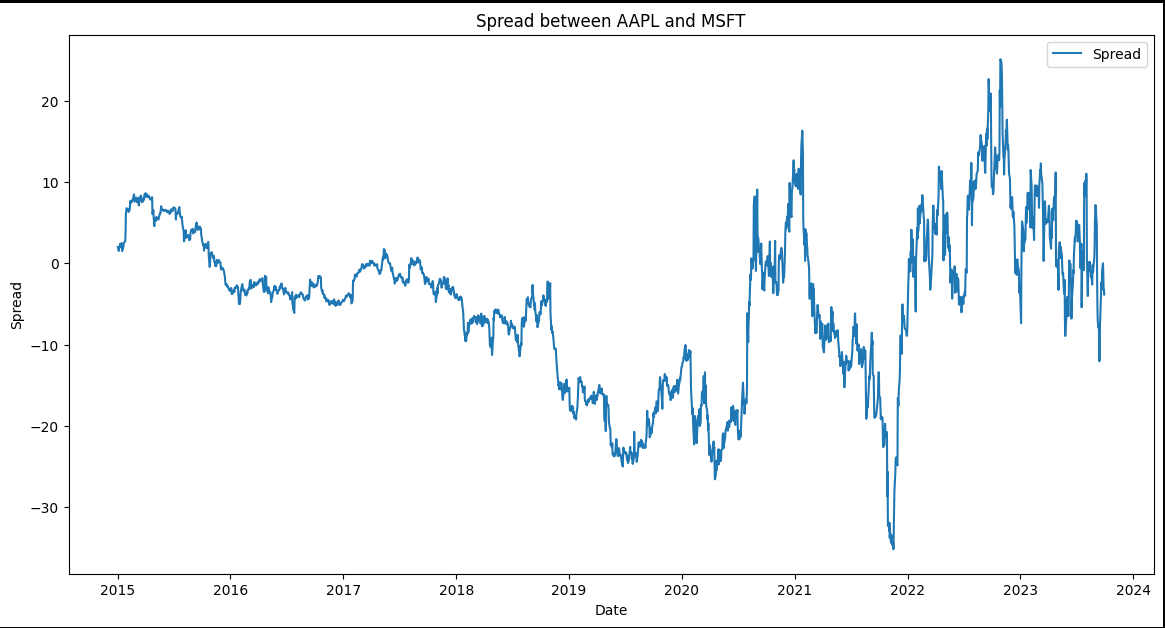
6. Calculating and Plotting the Spread

The spread is the difference between the prices of AAPL and MSFT, adjusted by the hedge ratio.

df['Spread'] = df[ticker1] - hedge_ratio * df[ticker2]

The spread shows how far apart the two stock prices have moved relative to each other. This is the key value that we’ll be trading based on. Pair trading strategies rely on mean reversion, meaning we expect the spread to eventually return to its historical average. Identifying when the spread is too wide or too narrow allows us to enter trades.

7. Z-Score Calculation

To quantify how far the spread is from its average, we calculate the Z-score.

df['Z_Score'] = (df['Spread'] - df['Spread_Mean']) / df['Spread_STD']

The Z-score measures how many standard deviations the current spread is from its mean. This helps us identify extreme deviations, which indicate potential trading opportunities.

When we use the Z-score, we can set thresholds to trigger buy and sell signals. A large positive or negative Z-score indicates that the spread is far from its average, suggesting it might revert.

8. Generating Buy/Sell Signals

We use the Z-score to generate signals for entering long or short positions.

df['Long_Signal'] = np.where(df['Z_Score'] <= -entry_threshold, 1, 0)
df['Short_Signal'] = np.where(df['Z_Score'] >= entry_threshold, -1, 0)
df['Positions'] = df['Long_Signal'] + df['Short_Signal']

Buy (long) signals are generated when the Z-score falls below a certain threshold, while sell (short) signals occur when the Z-score exceeds a positive threshold. These signals form the backbone of the strategy. It allows us to enter trades when the spread deviates significantly from the mean, assuming it will eventually revert.

9. Strategy Backtest and Performance

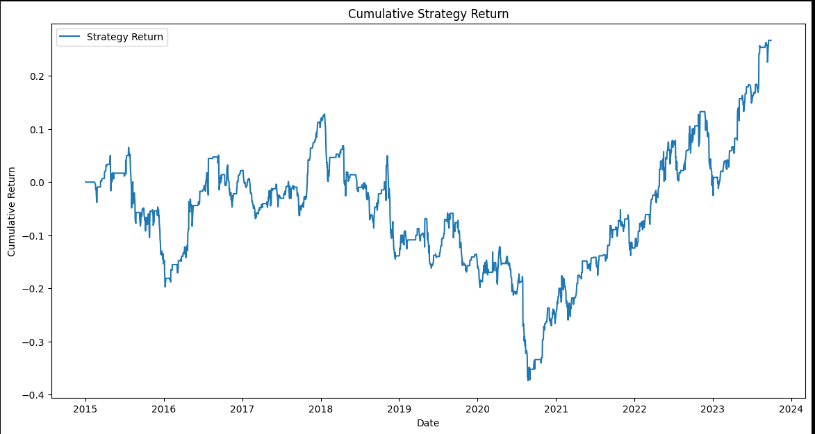
The next step is to calculate the cumulative returns of the strategy.

df['Strategy_Return'] = df['Positions'] * (df['Return_AAPL'] - hedge_ratio * df['Return_MSFT'])
df['Cumulative_Strategy_Return'] = (1 + df['Strategy_Return'].fillna(0)).cumprod() - 1

We backtest the strategy by applying our trading signals and calculating how profitable the trades would have been over time.

Backtesting shows us how the strategy would have performed historically, giving us insight into its potential profitability and robustness.

10. Transaction Costs and Net Strategy Return

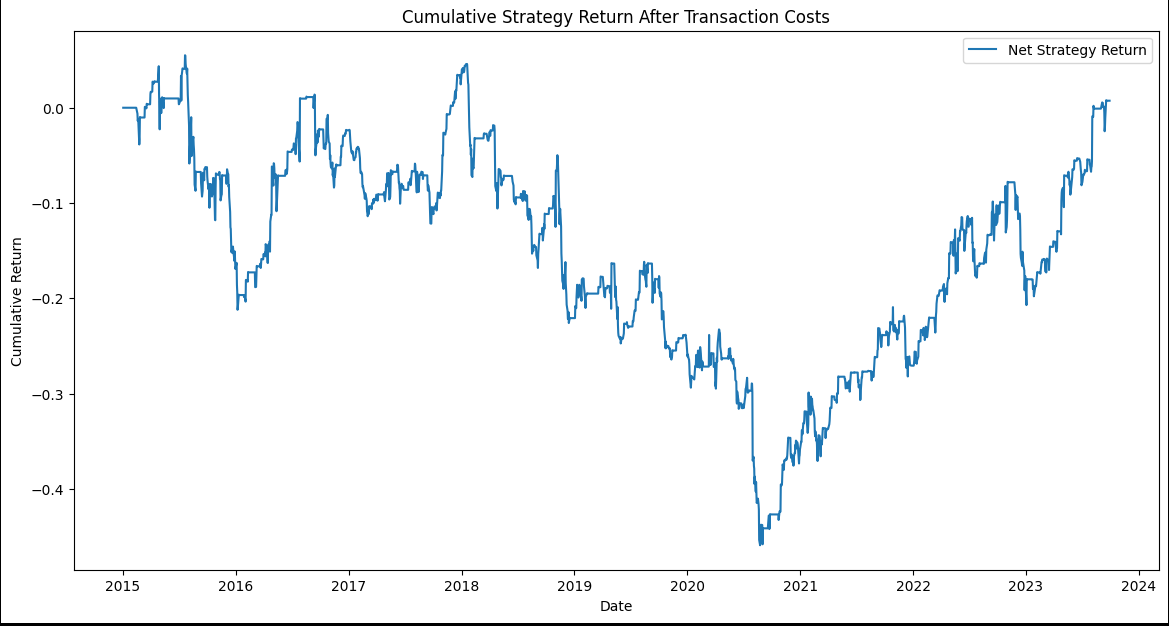
After accounting for transaction costs, we adjust the returns.

df['Strategy_Return_Net'] = df['Strategy_Return'] - df['Transaction_Costs']
df['Cumulative_Strategy_Return_Net'] = (1 + df['Strategy_Return_Net'].fillna(0)).cumprod() - 1

This step deducts transaction costs to provide a more realistic view of the strategy’s profitability.

Transaction costs can significantly reduce profits, especially in high-frequency trading strategies. Factoring in these costs ensures we have a clear understanding of the strategy’s viability.

11. Performance Metrics

Finally, we calculate key performance metrics.

print(f'Annualized Return: {annualized_return:.2%}')
print(f'Annualized Volatility: {annualized_volatility:.2%}')
print(f'Sharpe Ratio: {sharpe_ratio:.2f}')
print(f'Maximum Drawdown: {max_drawdown:.2%}')

Key performance metrics, including the Annualized Return, Volatility, Sharpe Ratio, and Maximum Drawdown, are calculated to assess the strategy’s effectiveness.

Result:

• Annualized Return: 3.94%

• Annualized Volatility: 15.70%

• Sharpe Ratio: 0.19

• Maximum Drawdown: 50.17%

These metrics help us evaluate the strategy’s risk and return profile. The Sharpe Ratio of 0.19 indicates low risk-adjusted returns, and the Maximum Drawdown of 50.17% shows significant risk exposure.

Understanding performance metrics like the Sharpe Ratio helps assess whether the strategy’s returns justify the risks involved. The high drawdown suggests the need for risk management improvements.

Conclusion:

Pair trading between Apple (AAPL) and Microsoft (MSFT) can be profitable, but it comes with risks like high drawdowns and a low Sharpe Ratio. This statistical arbitrage strategy centers on cointegration, hedge ratios, and Z-scores. To improve its performance, it’s important to optimize your entry and exit points and manage transaction costs. Pair trading offers a market-neutral way to profit from the dynamic relationship between these tech giants with careful execution.

Code Repository: https://github.com/gael55x/Linear-Arbitrage