
In partnership with

You Don’t Need to Be Technical. Just Informed

AI isn’t optional anymore—but coding isn’t required.
The AI Report gives business leaders the edge with daily insights, use cases, and implementation guides across ops, sales, and strategy.
Trusted by professionals at Google, OpenAI, and Microsoft.
👉 Get the newsletter and make smarter AI decisions.
🚀 Your Investing Journey Just Got Better: Premium Subscriptions Are Here! 🚀
It’s been 4 months since we launched our premium subscription plans at GuruFinance Insights, and the results have been phenomenal! Now, we’re making it even better for you to take your investing game to the next level. Whether you’re just starting out or you’re a seasoned trader, our updated plans are designed to give you the tools, insights, and support you need to succeed.
Here’s what you’ll get as a premium member:
Exclusive Trading Strategies: Unlock proven methods to maximize your returns.
In-Depth Research Analysis: Stay ahead with insights from the latest market trends.
Ad-Free Experience: Focus on what matters most—your investments.
Monthly AMA Sessions: Get your questions answered by top industry experts.
Coding Tutorials: Learn how to automate your trading strategies like a pro.
Masterclasses & One-on-One Consultations: Elevate your skills with personalized guidance.
Our three tailored plans—Starter Investor, Pro Trader, and Elite Investor—are designed to fit your unique needs and goals. Whether you’re looking for foundational tools or advanced strategies, we’ve got you covered.
Don’t wait any longer to transform your investment strategy. The last 4 months have shown just how powerful these tools can be—now it’s your turn to experience the difference.

Bitcoin’s Predicted Market Direction
Bitcoin’s price is known for its volatility, offering a valuable dataset for applying machine learning techniques to financial forecasting.
In this project, we focus on predicting whether Bitcoin’s price will move up or down the next day. We use historical price data and engineered technical indicators as input features.
This article covers the full process: data collection, preprocessing, feature engineering, feature selection, model training with a Random Forest classifier, and evaluating the model’s performance.
Smarter Investing Starts with Smarter News
The Daily Upside helps 1M+ investors cut through the noise with expert insights. Get clear, concise, actually useful financial news. Smarter investing starts in your inbox—subscribe free.
All the code used in this project is available on my GitHub repository for reference and reuse.
Installing Required Libraries
We begin by installing the Python packages used in this notebook. Each of these plays a critical role:
yfinance:to retrieve historical Bitcoin price data from Yahoo Finance.matplotlibandseaborn:for visualizing data and model performance.scikit-learn:to build, train, and evaluate the machine learning model.ta:to compute technical indicators like RSI and MACD.
%pip install yfinance matplotlib scikit-learn seaborn taImporting Libraries and Setting Plot Style
We then import all the relevant packages.
import yfinance as yf
import matplotlib.pyplot as plt
import seaborn as sns
from sklearn.ensemble import RandomForestClassifier
from sklearn.model_selection import train_test_split
from sklearn.metrics import classification_report, confusion_matrix
from sklearn.feature_selection import SelectKBest, f_classif
import ta
Downloading Historical Bitcoin Data
We use yfinance to download historical Bitcoin data from Yahoo Finance.
This dataset includes columns like Open, High, Low, Close, and Volume from Bitcoin’s inception in 2010 up to May 2025.
BTC-USDis the ticker for Bitcoin in US dollars.
data = yf.download("BTC-USD", start="2010-09-17", end="2025-05-19", auto_adjust=True)
data.head()
Selecting and Simplifying Columns
Some data providers like Yahoo Finance return multi-indexed columns. To make our dataset easier to work with, we:
Flatten the columns by selecting the top level.
Keep only the essential fields for price prediction:
Open,Close,Volume,Low, andHigh.
data.columns = data.columns.get_level_values(0)
data = data[['Open', 'Close', 'Volume', 'Low', 'High']]
Visualizing the Close Price
We display the historical closing price of Bitcoin.
plt.figure(figsize=(14, 6))
plt.plot(data.index, data['Close'], label='Close', color='blue')
plt.title('Close Price Over Time')
plt.xlabel('Date')
plt.ylabel('Close Price (USD)')
plt.legend()
plt.grid(True)
plt.savefig("Close.png")
plt.show()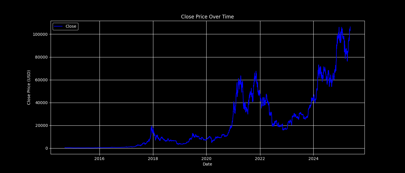
Bitcoin’s Closing Price Over Time
Creating the Target Variable
Our goal is to predict the direction of Bitcoin’s price the next day. So we create a binary target:
1if tomorrow's close is higher than today’s (price went up).0if it’s not (price went down or stayed the same).
We also drop rows with missing values caused by shifting.
data["Direction"] = (data["Close"].shift(-1) > data["Close"]).astype(int)
data.dropna(inplace=True)
Feature Engineering
To improve the predictive power of our model, we create new features derived from the raw price and volume data.
These engineered features help capture important market behaviors such as momentum, volatility, and trend strength that are not immediately obvious from the original data.
Return-Based Features
These features capture how much the price has changed over different time horizons. They help the model understand recent momentum and volatility:
Return_1d— daily return.Return_3d— 3-day return.Return_7d— 7-day return.
data["Return_1d"] = data["Close"].pct_change()
data["Return_3d"] = data["Close"].pct_change(3)
data["Return_7d"] = data["Close"].pct_change(7)
Price Range and Volatility Indicators
We compute features that quantify the price range and price volatility:
High_Low— difference between the daily high and low.Close_Open— intraday price movement.Volatility_7d— rolling 7-day standard deviation of closing prices.
data["High_Low"] = data["High"] - data["Low"]
data["Close_Open"] = data["Close"] - data["Open"]
data["Volatility_7d"] = data["Close"].rolling(7).std()
Moving Averages and Ratios
Moving averages smooth out short-term fluctuations and highlight trends.
We also compute the ratio between two moving averages to capture crossover patterns:
MA_5andMA_10— 5-day and 10-day moving averages.MA_ratio— relative trend strength over short and medium term.
data["MA_5"] = data["Close"].rolling(window=5).mean()
data["MA_10"] = data["Close"].rolling(window=10).mean()
data["MA_ratio"] = data["MA_5"] / data["MA_10"]
RSI Indicator
We use the ta library to calculate the Relative Strength Index (RSI), a momentum indicator that measures overbought or oversold conditions.
data["RSI"] = ta.momentum.RSIIndicator(data["Close"]).rsi()MACD Indicator
We calculate the MACD (Moving Average Convergence Divergence) and its signal line.
These are commonly used in trading strategies to detect shifts in momentum.
macd = ta.trend.MACD(data["Close"])
data["MACD"] = macd.macd()
data["MACD_signal"] = macd.macd_signal()
Volume-Based Features
Volume can confirm price movements. We compute:
Volume_Change— daily percentage change in volume.Volume_MA_5— 5-day moving average of volume.
data["Volume_Change"] = data["Volume"].pct_change()
data["Volume_MA_5"] = data["Volume"].rolling(5).mean()
Lag Features
Lagged features provide the model with recent values of price and volume:
Close_lag_1,Close_lag_2, etc. — yesterday’s and earlier close prices.Volume_lag_1, etc. — volume from previous days.
for lag in range(1, 4):
    data[f"Close_lag_{lag}"] = data["Close"].shift(lag)
    data[f"Volume_lag_{lag}"] = data["Volume"].shift(lag)
Calendar Features
We extract the day of the week and the month to help capture patterns like weekday effects or seasonal trends.
data["DayOfWeek"] = data.index.dayofweek  # Monday=0, Sunday=6
data["Month"] = data.index.month
Momentum and Rolling Extremes
These features help detect the strength and boundaries of trends:
Momentum_10— price change over the past 10 days.Rolling_Max_10,Rolling_Min_10— recent highest and lowest close prices.
data["Momentum_10"] = data["Close"] - data["Close"].shift(10)
data["Rolling_Max_10"] = data["Close"].rolling(10).max()
data["Rolling_Min_10"] = data["Close"].rolling(10).min()
Dropping Missing Values
All the above transformations may introduce NaN values. We remove these rows to clean the dataset.
data.dropna(inplace=True)Preparing the Feature Matrix and Target
We separate our dataset into:
X: feature matrix (all columns except the target).y: target variable indicating if the price went up (1) or not (0).
X = data.drop(columns=["Direction"])
y = data["Direction"]
Feature Selection with SelectKBest
We use SelectKBest with the ANOVA F-test to select the 10 most informative features.
This helps reduce noise and improve model performance.
selector = SelectKBest(score_func=f_classif, k=10)
X_selected = selector.fit_transform(X, y)
Visualizing Feature Importance
We plot the F-scores of the top 10 selected features to understand which ones contributed most to the target.
# Get scores and mask of selected features
scores = selector.scores_
selected_mask = selector.get_support()  # boolean mask of selected features
selected_feature_names = X.columns[selected_mask]

# Plot
plt.figure(figsize=(14, 6))
plt.barh(selected_feature_names, scores[selected_mask], color="teal")
plt.xlabel("F-score")
plt.title("Top 5 Selected Features by F-score (SelectKBest)")
plt.gca().invert_yaxis()  # optional: put highest on top
plt.tight_layout()
plt.savefig("feature_importance.png")
plt.show()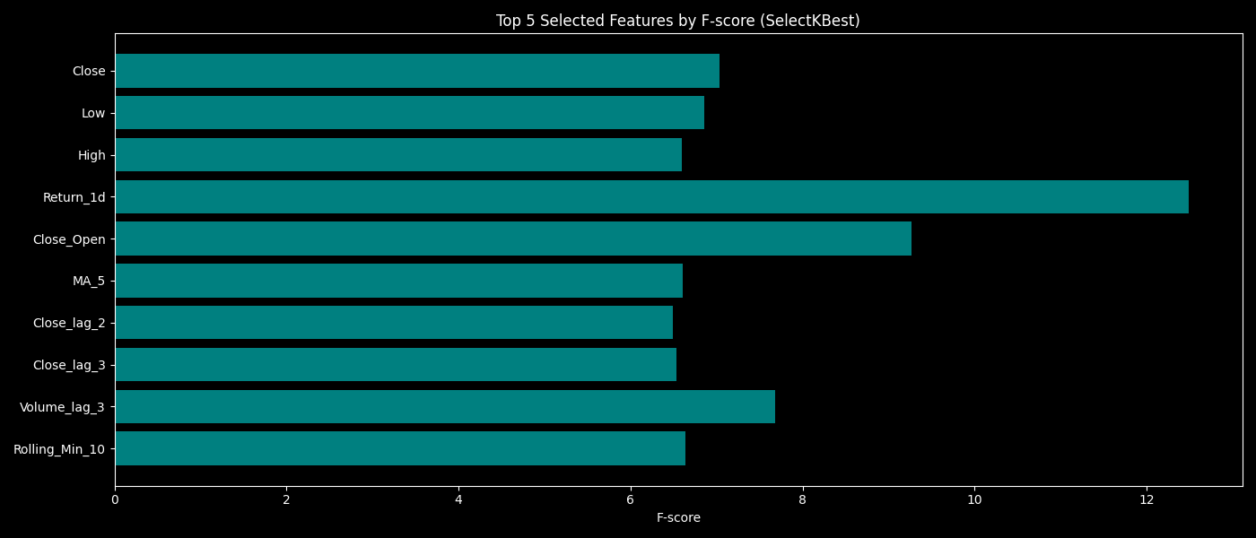
Feature Importance from SelectKBest Feature Selection
Splitting the Data
We split the dataset into training and testing sets using an 80/20 ratio. Note: shuffle=False is used to preserve the time-series order.
X_train, X_test, y_train, y_test = train_test_split(
    X_selected, y, test_size=0.2, random_state=42, shuffle=False
)
Training the Random Forest Model
We train a RandomForestClassifier to learn the relationship between features and the target.
class_weight='balanced'ensures that the model accounts for class imbalance if any.
model = RandomForestClassifier(n_estimators=100, random_state=42, class_weight='balanced')
model.fit(X_train, y_train)
Generating Predictions and Evaluating Performance
We make predictions on the test set and print a classification report including precision, recall, and F1-score.
y_pred = model.predict(X_test)
print(classification_report(y_test, y_pred))
precision recall f1-score support
0 0.51 0.78 0.62 380
1 0.57 0.28 0.38 393
accuracy 0.53 773
macro avg 0.54 0.53 0.50 773
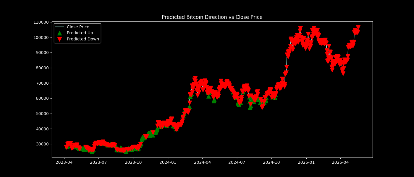
weighted avg 0.54 0.53 0.50 773Visualizing Predictions vs Market Movements
This plot overlays model predictions on Bitcoin’s closing price:
Green triangles indicate days where the model predicted an upward movement.
Red triangles indicate predicted downward movements.
plt.figure(figsize=(14,6))
plt.plot(data.index[-len(y_test):], data["Close"][-len(y_test):], label='Close Price')
plt.plot(data.index[-len(y_test):][y_pred == 1], data["Close"][-len(y_test):][y_pred == 1], '^', markersize=10, color='g', label='Predicted Up')
plt.plot(data.index[-len(y_test):][y_pred == 0], data["Close"][-len(y_test):][y_pred == 0], 'v', markersize=10, color='r', label='Predicted Down')
plt.title("Predicted Bitcoin Direction vs Close Price")
plt.legend()
plt.savefig("predicted_market_direction.png")
plt.show()
Predicted Bitcoin Direction vs Close Price
Confusion Matrix
A confusion matrix gives a snapshot of how many predictions were correct and incorrect. It distinguishes:
True positives (correctly predicted ups).
True negatives (correctly predicted downs).
False positives and false negatives.
cm = confusion_matrix(y_test, y_pred)
sns.heatmap(cm, annot=True, fmt='d', cmap='Blues')
plt.xlabel('Predicted')
plt.ylabel('Actual')
plt.title('Confusion Matrix')
plt.savefig("confusion_matrix.png")
plt.show()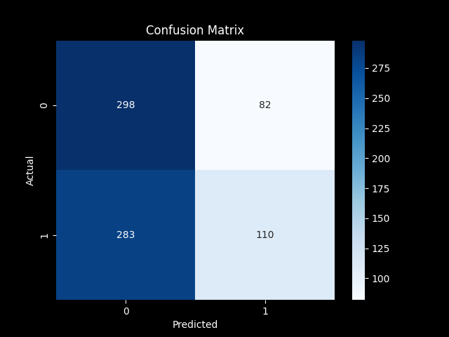
Confusion Matrix
This project demonstrates how machine learning and thoughtful feature engineering can be used to predict the direction of Bitcoin’s price.
While our model makes use of simple technical indicators and historical data, real-world trading strategies would require additional considerations such as transaction costs, slippage, and risk management.