
In partnership with

What Top Execs Read Before the Market Opens

The Daily Upside was founded by investment professionals to arm decision-makers with market intelligence that goes deeper than headlines. No filler. Just concise, trusted insights on business trends, deal flow, and economic shifts—read by leaders at top firms across finance, tech, and beyond.
🚀 Your Investing Journey Just Got Better: Premium Subscriptions Are Here! 🚀
It’s been 4 months since we launched our premium subscription plans at GuruFinance Insights, and the results have been phenomenal! Now, we’re making it even better for you to take your investing game to the next level. Whether you’re just starting out or you’re a seasoned trader, our updated plans are designed to give you the tools, insights, and support you need to succeed.
Here’s what you’ll get as a premium member:
Exclusive Trading Strategies: Unlock proven methods to maximize your returns.
In-Depth Research Analysis: Stay ahead with insights from the latest market trends.
Ad-Free Experience: Focus on what matters most—your investments.
Monthly AMA Sessions: Get your questions answered by top industry experts.
Coding Tutorials: Learn how to automate your trading strategies like a pro.
Masterclasses & One-on-One Consultations: Elevate your skills with personalized guidance.
Our three tailored plans—Starter Investor, Pro Trader, and Elite Investor—are designed to fit your unique needs and goals. Whether you’re looking for foundational tools or advanced strategies, we’ve got you covered.
Don’t wait any longer to transform your investment strategy. The last 4 months have shown just how powerful these tools can be—now it’s your turn to experience the difference.

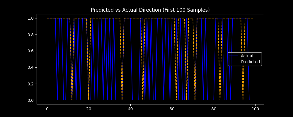
Predicted vs Actual Direction Chart
Stock prices change for many reasons. News, earnings reports, market trends, and investor behavior all play a role.
Most of these factors are unpredictable. But sometimes, patterns in historical prices offer small clues about what might happen next.
This project tests whether a Long Short-Term Memory (LSTM) model can detect those clues. We are not trying to predict exact prices. The goal is to classify the next week’s price movement as either up or down. That makes it a binary classification problem.
We use data from 19 large tech companies, with weekly price and volume information going back more than 20 years.
Each data sample is a short sequence of past observations. The model tries to learn from these sequences and predict the direction of the next move.
You Deserve to Feel Better — Start Therapy Completely Free
BetterHelp is making therapy more accessible than ever this May. For a limited time, get your first week free and talk to a licensed therapist from the comfort of your home.
94% of users say they feel better after starting therapy on BetterHelp, and 93% are matched with someone who fits their needs. You can chat, call, or message your therapist whenever it works for you.
There’s no pressure, no commitment—just real support, on your terms.
Why Use LSTM
LSTM networks are designed to work with sequence data. They are especially good at learning from patterns that develop over time, which is exactly what stock price data looks like.
We use weekly data instead of daily data to reduce noise. Weekly trends are less affected by short-term market fluctuations, allowing the model to focus on longer-term patterns with less noise
Financial markets are chaotic and constantly changing. That is what makes this problem interesting. We are testing how much, if anything, a deep learning model can learn from historical data in a real-world setting.
Set Up the Environment
We use the following stack:
yfinance– To fetch historical weekly stock data.scikit-learn– For preprocessing, scaling, and model evaluation.TensorFlow/Keras– To build and train the LSTM neural network.matplotlib&seaborn– For visualization.
In your python environment, install them using:
%pip install yfinance matplotlib scikit-learn tensorflow seabornOnce the libraries are successfully installed, we import them as follows:
# Standard libraries
import numpy as np
import yfinance as yf
import matplotlib.pyplot as plt
import seaborn as sns

# Scikit-learn
from sklearn.preprocessing import MinMaxScaler
from sklearn.model_selection import train_test_split
from sklearn.metrics import confusion_matrix, classification_report

# TensorFlow/Keras
from tensorflow.keras.models import Sequential
from tensorflow.keras.layers import LSTM, Dense, Dropout

# Plotting style
plt.style.use('dark_background')
Data Collection and Preprocessing
We begin by specifying the list of stock tickers we’ll use for this experiment.
These are 19 major tech-related companies with liquid and volatile stocks, making them ideal for pattern discovery in price movements.
tickers = [
    'AAPL', 'MSFT', 'GOOGL', 'AMZN', 'META', 'NVDA', 'TSLA', 'AMD',
    'INTC', 'CRM', 'ADBE', 'ORCL', 'SHOP', 'UBER', 'LYFT',
    'NFLX', 'TWLO', 'SNOW', 'PLTR'
]
Create Input Sequences
Next, we define a utility function to convert raw data into input sequences suitable for training an LSTM model.
Each sequence is a sliding window of 10 time steps (weeks), and the corresponding label is the binary target that immediately follows the sequence.
def create_sequences(data, target, sequence_length=10):
    X, y = [], []
    for i in range(len(data) - sequence_length):
        X.append(data[i:i + sequence_length])
        y.append(target[i + sequence_length])
    return np.array(X), np.array(y)
This function allows the model to learn temporal patterns in stock movement over a fixed-length context.
We now loop through each ticker, download its historical weekly data from Yahoo Finance, and prepare it for model training:
sequence_length = 10
all_X, all_y = [], []

for ticker in tickers:
    df = yf.download(ticker, start='2000-01-01', end='2024-12-31', interval='1wk')[['Open', 'High', 'Low', 'Close', 'Volume']]
    df.dropna(inplace=True)

    # Binary target: price will go up next week
    df['Target'] = np.where(df['Close'].shift(-1) > df['Close'], 1, 0)
    df.dropna(inplace=True)

    # Feature scaling
    scaler = MinMaxScaler()
    features = scaler.fit_transform(df[['Open', 'High', 'Low', 'Close', 'Volume']])
    X, y = create_sequences(features, df['Target'].values, sequence_length=sequence_length)
    all_X.append(X)
    all_y.append(y)
We use weekly data to smooth out short-term noise.
The target variable is binary:
1if the next week’s close is higher than the current,0otherwise.Features are scaled between 0 and 1 using
MinMaxScalerfor better neural network performance.For each ticker, sequences and corresponding labels are created and stored.
After processing all tickers, we merge all the sequences into a single dataset:
# Combine all stocks' sequences
X_all = np.concatenate(all_X, axis=0)
y_all = np.concatenate(all_y, axis=0)
This gives us a large pool of sequences sampled from diverse stocks, helping the model generalize better.
Data Split
To properly prepare the data for training and evaluation, we first split the dataset into three sets: training, validation, and testing. We used a common 70–15–15 split to ensure a balanced distribution:
# First split: train vs (validation + test)
X_train, X_temp, y_train, y_temp = train_test_split(
    X_all, y_all, test_size=0.3, random_state=42, shuffle=True
)

# Second split: validation vs test
X_val, X_test, y_val, y_test = train_test_split(
    X_temp, y_temp, test_size=0.5, random_state=42, shuffle=True
)
This means 70% of the data is used for training, 15% for validation, and 15% for testing.
Since each sequence is independent, shuffling does not violate the temporal integrity of the data.
This split ensures that we have enough data for training while maintaining proper evaluation sets for model performance.
Building the LSTM Model
For this model, we opt for a three-layer LSTM architecture, incorporating dropout layers for regularization:
model = Sequential([
    LSTM(100, return_sequences=True, input_shape=(X_train.shape[1], X_train.shape[2])),
    Dropout(0.3),
    LSTM(100, return_sequences=True),
    Dropout(0.3),
    LSTM(100),
    Dropout(0.3),
    Dense(1, activation='sigmoid')
])
The three LSTM layers are designed to capture more intricate temporal dependencies in the stock price data. By stacking LSTM layers, the model can learn both short-term and long-term patterns from the sequential data.
The dropout layers, each with a 30% rate, help mitigate overfitting by randomly disabling a fraction of neurons during training, ensuring that the model generalizes better to unseen data.
Finally, the sigmoid activation function in the output layer makes it suitable for a binary classification task, predicting whether the stock price will move up (1) or down (0) in the next week.
Compile the model:
model.compile(loss='binary_crossentropy', optimizer='adam', metrics=['accuracy'])
model.summary()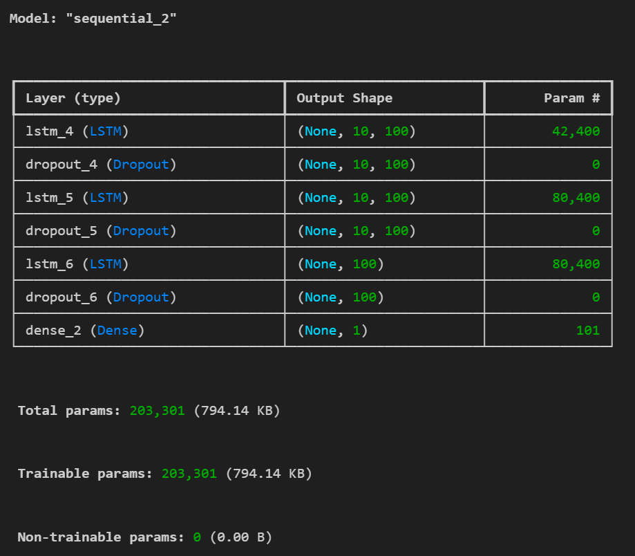
LSTM Model Architecture Summary
Training the Model
We train the model for 100 epochs with validation on the validation set:
history = model.fit(
    X_train, y_train,
    epochs=100,
    batch_size=32,
    validation_data=(X_val, y_val),
    verbose=1
)
Evaluating Performance
Evaluate accuracy on the test set:
loss, accuracy = model.evaluate(X_test, y_test)
print(f"Test Accuracy: {accuracy:.4f}")Output:
Test Accuracy: 0.5241We also visualize training history:
plt.figure(figsize=(12, 4))

# Loss plot
plt.subplot(1, 2, 1)
plt.plot(history.history['loss'], label='Train Loss', color='blue')
plt.plot(history.history['val_loss'], label='Val Loss', color='orange')
plt.title('Loss over Epochs')
plt.xlabel('Epoch')
plt.ylabel('Loss')
plt.legend()

# Accuracy plot
plt.subplot(1, 2, 2)
plt.plot(history.history['accuracy'], label='Train Accuracy', color='blue')
plt.plot(history.history['val_accuracy'], label='Val Accuracy', color='orange')
plt.title('Accuracy over Epochs')
plt.xlabel('Epoch')
plt.ylabel('Accuracy')
plt.legend()
plt.tight_layout()
plt.savefig('loss_accuracy.png')
plt.show()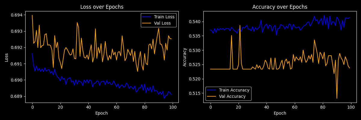
Loss/Accuracy Training Plots
These plots reveal if the model is overfitting (diverging val loss) or underfitting (both losses high).
Predictions and Reports
Convert predicted probabilities to binary values:
y_pred_probs = model.predict(X_test)
y_pred = (y_pred_probs > 0.5).astype(int).flatten()
y_true = y_test.flatten()
Print a detailed classification report:
print(classification_report(y_test, y_pred, target_names=['Down (0)', 'Up (1)']))Classification Report:
precision recall f1-score support
Down (0) 0.44 0.07 0.12 1189
Up (1) 0.53 0.92 0.67 1358
accuracy 0.52 2547
macro avg 0.49 0.50 0.40 2547
weighted avg 0.49 0.52 0.42 2547Visualize the confusion matrix:
cm = confusion_matrix(y_true, y_pred)

plt.figure(figsize=(6, 5))
sns.heatmap(cm, annot=True, fmt='d', cmap='Blues', xticklabels=['Down (0)', 'Up (1)'], yticklabels=['Down (0)', 'Up (1)'])
plt.xlabel('Predicted')
plt.ylabel('Actual')
plt.title('Confusion Matrix')
plt.savefig('confusion_matrix.png')
plt.show()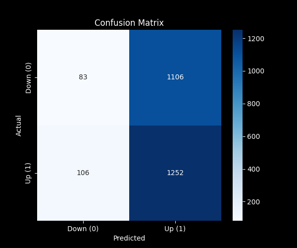
Confusion Matrix
Compare actual vs predicted direction:
plt.figure(figsize=(10, 4))
plt.plot(y_test[:100], label='Actual', color='blue')
plt.plot(y_pred[:100], label='Predicted', color='orange', linestyle='--')
plt.legend()
plt.title('Predicted vs Actual Direction (First 100 Samples)')
plt.savefig('predicted_vs_actual.png')
plt.show()
Predicted vs Actual Price Direction Chart
Limitations and Future Improvements
This project has several constraints worth noting. Stock market data is noisy, non-stationary, and semi-efficient — limiting how much predictive power we can extract from OHLCV data alone.
We used a binary classification target (up or down), which simplifies the task but still poses challenges in such volatile environments.
Additionally, our features were limited to price and volume, leaving out technical indicators, sentiment signals, or macroeconomic variables that could enhance model performance.
Metrics like accuracy may also be misleading in imbalanced datasets; alternative metrics like F1-score or ROC-AUC should be considered.
To improve the model, one could experiment with more informative features (e.g., RSI, MACD), integrate news sentiment or economic data, and explore more advanced architectures like transformers or multi-task learning setups.
This project shows how we can apply LSTMs to financial data to model price direction using only historical prices.
While promising, this approach has real-world limitations. The market is complex, and a simple neural network may not unlock its secrets — but it’s a powerful exercise in time series modeling, preprocessing, and deep learning application.