Your job called—it wants better business news

Welcome to Morning Brew—the world’s most engaging business newsletter. Seriously, we mean it.

Morning Brew’s daily email keeps professionals informed on the business news that matters, but with a twist—think jokes, pop culture, quick writeups, and anything that makes traditionally dull news actually enjoyable.

It’s 100% free—so why not give it a shot? And if you decide you’d rather stick with dry, long-winded business news, you can always unsubscribe.

Check it out

🚀 Your Investing Journey Just Got Better: Premium Subscriptions Are Here! 🚀

It’s been 4 months since we launched our premium subscription plans at GuruFinance Insights, and the results have been phenomenal! Now, we’re making it even better for you to take your investing game to the next level. Whether you’re just starting out or you’re a seasoned trader, our updated plans are designed to give you the tools, insights, and support you need to succeed.

Here’s what you’ll get as a premium member:

• Exclusive Trading Strategies: Unlock proven methods to maximize your returns.

• In-Depth Research Analysis: Stay ahead with insights from the latest market trends.

• Ad-Free Experience: Focus on what matters most—your investments.

• Monthly AMA Sessions: Get your questions answered by top industry experts.

• Coding Tutorials: Learn how to automate your trading strategies like a pro.

• Masterclasses & One-on-One Consultations: Elevate your skills with personalized guidance.

Our three tailored plans—Starter Investor, Pro Trader, and Elite Investor—are designed to fit your unique needs and goals. Whether you’re looking for foundational tools or advanced strategies, we’ve got you covered.

Don’t wait any longer to transform your investment strategy. The last 4 months have shown just how powerful these tools can be—now it’s your turn to experience the difference.

👉 Explore Premium Plans Now

A rigorous approach to measuring and managing financial risk hinges on understanding how expected returns, volatility, and the co‑movement of assets interact — and how to combine assets into portfolios that optimize these trade‑offs.

Python Setup & Data Fetching First, we’ll set up our Python environment and fetch some stock data using yfinance.

Python

import yfinance as yf
import pandas as pd
import numpy as np

# Define the tickers and the time period for historical data
tickers = ['AAPL', 'MSFT', 'GOOG']
market_index = '^GSPC' # S&P 500
start_date = '2020-01-01'
end_date = '2023-12-31'

# Download historical stock data for 'Adj Close' prices
# 'Adj Close' accounts for dividends and stock splits
try:
    data = yf.download(tickers, start=start_date, end=end_date, auto_adjust=False)['Adj Close']
    market_data = yf.download(market_index, start=start_date, end=end_date, auto_adjust=False)['Close']
except Exception as e:
    print(f"Error downloading data: {e}")
    data = pd.DataFrame() # Create empty dataframe to avoid further errors
    market_data = pd.Series(dtype='float64') # Create empty series

# Display the first few rows of the data
print("Stock Data:")
print(data.head())
print("\nMarket Data (S&P 500):")
print(market_data.head())

Stock Data:
Ticker           AAPL       GOOG        MSFT
Date                                        
2020-01-02  72.716072  68.046196  153.323242
2020-01-03  72.009117  67.712280  151.414124
2020-01-06  72.582916  69.381874  151.805511
2020-01-07  72.241524  69.338585  150.421371
2020-01-08  73.403648  69.884995  152.817352

Market Data (S&P 500):
Ticker            ^GSPC
Date                   
2020-01-02  3257.850098
2020-01-03  3234.850098
2020-01-06  3246.280029
2020-01-07  3237.179932
2020-01-08  3253.050049

1. Expected Return and Volatility

Pay No Interest Until Nearly 2027 AND Earn 5% Cash Back

Use a 0% intro APR card to pay off debt.
Transfer your balance and avoid interest charges.
This top card offers 0% APR into 2027 + 5% cash back!

Learn How To Apply Now

1.1 Portfolio Return
If you invest fractions wᵢ of your wealth in n assets whose individual returns are rᵢ, the portfolio return over a period is

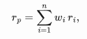
and its expectation is

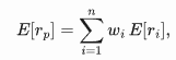
with ∑wᵢ=1.

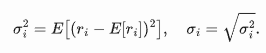
1.2 Portfolio Volatility
Risk is measured by standard deviation. For asset i,

Portfolio variance blends individual variances and covariances:

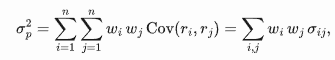
1.3 Correlations

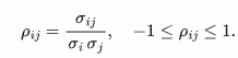
Less-than-perfect correlations (ρ<1) enable diversification and reduce σₚ.

Python

# Calculate daily returns
asset_returns = asset_data.pct_change().dropna()
market_returns = market_data.pct_change().dropna()

print("Asset Daily Returns (head):")
print(asset_returns.head())
print("\nMarket Daily Returns (head):")
print(market_returns.head())

# Calculate mean daily returns for each asset (proxy for E[r_i])
mean_daily_returns = asset_returns.mean()
print("\nMean Daily Returns:")
print(mean_daily_returns)

# Calculate expected portfolio return (daily)
expected_portfolio_return_daily = np.sum(mean_daily_returns * weights)
print(f"\nExpected Daily Portfolio Return: {expected_portfolio_return_daily:.6f}")

# Annualize the expected portfolio return (assuming 252 trading days)
annual_trading_days = 252
expected_portfolio_return_annual = expected_portfolio_return_daily * annual_trading_days
print(f"Expected Annual Portfolio Return: {expected_portfolio_return_annual:.4f}")

# Calculate daily covariance matrix of asset returns
cov_matrix_daily = asset_returns.cov()
print("\nDaily Covariance Matrix of Asset Returns:")
print(cov_matrix_daily)

# Calculate portfolio variance (daily)
portfolio_variance_daily = np.dot(weights.T, np.dot(cov_matrix_daily, weights))
print(f"\nDaily Portfolio Variance: {portfolio_variance_daily:.8f}")

# Calculate portfolio volatility (standard deviation - daily)
portfolio_volatility_daily = np.sqrt(portfolio_variance_daily)
print(f"Daily Portfolio Volatility: {portfolio_volatility_daily:.6f}")

# Annualize portfolio volatility
portfolio_volatility_annual = portfolio_volatility_daily * np.sqrt(annual_trading_days)
print(f"Annual Portfolio Volatility: {portfolio_volatility_annual:.4f}")

# Calculate daily correlation matrix
correlation_matrix = asset_returns.corr()
print("\nDaily Correlation Matrix of Asset Returns:")
print(correlation_matrix)

Asset Daily Returns (head):
Ticker          AAPL      GOOG      MSFT
Date                                    
2020-01-03 -0.009722 -0.004907 -0.012452
2020-01-06  0.007968  0.024657  0.002585
2020-01-07 -0.004703 -0.000624 -0.009118
2020-01-08  0.016087  0.007880  0.015928
2020-01-09  0.021241  0.011044  0.012493

Market Daily Returns (head):
Ticker         ^GSPC
Date                
2020-01-03 -0.007060
2020-01-06  0.003533
2020-01-07 -0.002803
2020-01-08  0.004902
2020-01-09  0.006655

Mean Daily Returns:
Ticker
AAPL    0.001187
GOOG    0.000942
MSFT    0.001095
dtype: float64

Expected Daily Portfolio Return: 0.001075
Expected Annual Portfolio Return: 0.2708

Daily Covariance Matrix of Asset Returns:
Ticker      AAPL      GOOG      MSFT
Ticker                              
AAPL    0.000447  0.000307  0.000338
GOOG    0.000307  0.000444  0.000333
MSFT    0.000338  0.000333  0.000422

Daily Portfolio Variance: 0.00036328
Daily Portfolio Volatility: 0.019060
Annual Portfolio Volatility: 0.3026

Daily Correlation Matrix of Asset Returns:
Ticker      AAPL      GOOG      MSFT
Ticker                              
AAPL    1.000000  0.689177  0.777003
GOOG    0.689177  1.000000  0.769150
MSFT    0.777003  0.769150  1.000000

2. Estimating Parameters via Maximum Likelihood

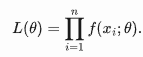
To calibrate models to observed return series, Maximum Likelihood Estimation (MLE) finds parameter values θ that maximize the probability of the data.

• Likelihood Function:
  For independent observations x1,…,xn with density f(x;θ),

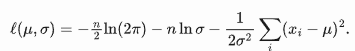
• Log‑Likelihood:

which is maximized by solving ∂ℓ/∂θj=0 for each parameter .

• Example (Normal Distribution):
  If xi∼N(μ,σ2),

• First‑order conditions yield

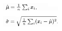
Python

# For demonstration, let's calculate sample mean and std for AAPL's daily returns
# These are the MLE estimates if we assume returns are normally distributed.
aapl_returns = asset_returns['AAPL']
mu_hat_aapl = aapl_returns.mean() # MLE for mu
sigma_hat_aapl = aapl_returns.std(ddof=0) # MLE for sigma (ddof=0 for population std)

print(f"\nMLE estimate for AAPL daily return mean (mu_hat): {mu_hat_aapl:.6f}")
print(f"MLE estimate for AAPL daily return std (sigma_hat): {sigma_hat_aapl:.6f}")

MLE estimate for AAPL daily return mean (mu_hat): 0.001187
MLE estimate for AAPL daily return std (sigma_hat): 0.021135

3. The Risk–Return Trade‑Off

3.1 Normality Assumption
Many models assume returns are normally distributed (μ,σ,), so that

• about 68% of outcomes lie within one σof μ,

• about 95% lie within two σ.

3.2 Efficient Frontier
Harry Markowitz showed that, when plotting portfolios’ (σp,E[rp]), the upper boundary (the efficient frontier) comprises portfolios offering the highest return for each risk level.

4. Constructing Optimal Portfolios

To find the minimum‑variance portfolio delivering a target expected return μₚ:

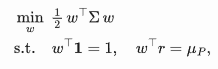
where r is the vector of expected asset returns and Σ their covariance matrix. Introducing Lagrange multipliers leads to explicit weights

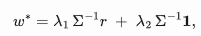
with

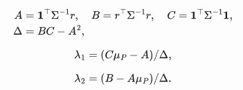
Plotting σₚ vs. μₚ yields a curve, upper part of which is the efficient frontier.

import matplotlib.pyplot as plt

# Ensure mean_daily_returns and cov_matrix_daily are available and not empty
if 'mean_daily_returns' in locals() and not mean_daily_returns.empty and \
   'cov_matrix_daily' in locals() and not cov_matrix_daily.empty and \
   len(mean_daily_returns) == cov_matrix_daily.shape[0] and \
   len(tickers) == len(mean_daily_returns): # Check consistency

    r = mean_daily_returns.values # Vector of mean daily returns
    Sigma = cov_matrix_daily.values # Covariance matrix of daily returns
    num_assets_frontier = len(r)
    ones = np.ones(num_assets_frontier)

    try:
        Sigma_inv = np.linalg.inv(Sigma) # Inverse of the covariance matrix

        # Calculate A, B, C, and Delta
        A = ones.T @ Sigma_inv @ r
        B = r.T @ Sigma_inv @ r
        C = ones.T @ Sigma_inv @ ones
        Delta = B * C - A**2

        if Delta == 0:
            print("Delta is zero. Cannot calculate efficient frontier using this method (assets might be perfectly correlated or other degeneracy).")
        else:
            # Determine a range of target expected portfolio returns (mu_P) for plotting
            # We'll go from the Global Minimum Variance Portfolio return upwards
            mu_gmvp_daily = A / C # Expected return of the Global Minimum Variance Portfolio (daily)
            
            # Let's target a range of returns from GMVP up to the max individual asset return (or a bit higher)
            min_target_return_daily = mu_gmvp_daily
            max_target_return_daily = np.max(r) * 1.5 # Go a bit beyond the max individual asset return
            
            # If max_target_return_daily is less than min_target_return_daily (e.g. if max(r)*1.5 < A/C)
            # adjust max_target_return_daily to be slightly above min_target_return_daily
            if max_target_return_daily <= min_target_return_daily:
                max_target_return_daily = min_target_return_daily * (1.05 if min_target_return_daily > 0 else 0.95) # 5% more or less depending on sign
                if max_target_return_daily == min_target_return_daily : # if mu_gmvp is zero
                     max_target_return_daily = 0.001 # a small positive value if mu_gmvp_daily is 0

            target_returns_daily = np.linspace(min_target_return_daily, max_target_return_daily, 100)
            
            portfolio_volatilities_daily = []
            portfolio_returns_daily_plot = [] # Store actual mu_p used for plotting
            all_weights = []

            for mu_P_daily in target_returns_daily:
                lambda1 = (C * mu_P_daily - A) / Delta
                lambda2 = (B - A * mu_P_daily) / Delta
                
                w_star = lambda1 * (Sigma_inv @ r) + lambda2 * (Sigma_inv @ ones)
                
                # Calculate portfolio variance and standard deviation for this mu_P_daily
                # var_p_daily = w_star.T @ Sigma @ w_star # This should be (C*mu_P_daily^2 - 2*A*mu_P_daily + B) / Delta
                var_p_daily = (C * (mu_P_daily**2) - 2 * A * mu_P_daily + B) / Delta # Variance of portfolio for a given mu_P
                
                # Due to numerical precision, var_p_daily could be extremely small negative. Take abs or max with 0.
                if var_p_daily < 0: var_p_daily = 0 # Avoid math domain error with sqrt

                std_p_daily = np.sqrt(var_p_daily)
                
                portfolio_volatilities_daily.append(std_p_daily)
                portfolio_returns_daily_plot.append(mu_P_daily) # This is our target return
                all_weights.append(w_star)

            # Convert to numpy arrays for easier annualization
            portfolio_volatilities_daily = np.array(portfolio_volatilities_daily)
            portfolio_returns_daily_plot = np.array(portfolio_returns_daily_plot)

            # Annualize for plotting
            portfolio_returns_annual_plot = portfolio_returns_daily_plot * annual_trading_days
            portfolio_volatilities_annual = portfolio_volatilities_daily * np.sqrt(annual_trading_days)

            # Plotting the Efficient Frontier
            plt.figure(figsize=(10, 6))
            plt.plot(portfolio_volatilities_annual, portfolio_returns_annual_plot, 'b-', lw=2, label='Efficient Frontier')
            
            # Plot individual assets
            asset_volatilities_annual = np.sqrt(np.diag(Sigma)) * np.sqrt(annual_trading_days)
            asset_returns_annual = r * annual_trading_days
            plt.scatter(asset_volatilities_annual, asset_returns_annual, marker='o', s=50, label='Individual Assets')
            for i, ticker in enumerate(tickers): # Use asset_tickers from global scope
                 plt.text(asset_volatilities_annual[i], asset_returns_annual[i], f' {ticker}', fontsize=9)

            # Plot Global Minimum Variance Portfolio (GMVP)
            sigma_gmvp_daily = np.sqrt(1/C)
            mu_gmvp_annual = mu_gmvp_daily * annual_trading_days
            sigma_gmvp_annual = sigma_gmvp_daily * np.sqrt(annual_trading_days)
            plt.scatter(sigma_gmvp_annual, mu_gmvp_annual, marker='*', color='red', s=150, label='Global Minimum Variance Portfolio (GMVP)')
            plt.text(sigma_gmvp_annual, mu_gmvp_annual, ' GMVP', fontsize=9)


            plt.title('Efficient Frontier')
            plt.xlabel('Annualized Volatility (Standard Deviation)')
            plt.ylabel('Annualized Expected Return')
            plt.legend()
            plt.grid(True)
            plt.show()

            # You can also find the portfolio with the highest Sharpe Ratio (Tangency Portfolio)
            # This requires a risk-free rate and typically numerical optimization,
            # or solving for specific lambdas if a risk-free asset is introduced analytically.
            # For now, we'll just plot the frontier of risky assets.

    except np.linalg.LinAlgError:
        print("Covariance matrix is singular or not invertible. Cannot calculate efficient frontier.")
    except Exception as e:
        print(f"An error occurred during efficient frontier calculation: {e}")

elif not ('mean_daily_returns' in locals() and 'cov_matrix_daily' in locals()):
    print("Mean returns or covariance matrix not available. Skipping efficient frontier calculation.")
elif mean_daily_returns.empty or cov_matrix_daily.empty:
    print("Mean returns or covariance matrix is empty. Skipping efficient frontier calculation.")
else:
    print("Data inconsistency. Skipping efficient frontier calculation. Check dimensions of returns and covariance matrix vs asset_tickers.")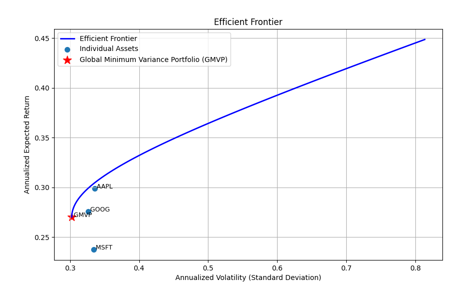

5. The Market Price of Risk

The market price of risk λ is the extra expected return per unit of risk:

where rf is the risk‑free rate. In derivatives theory, no‑arbitrage arguments show that for any claim with drift μ and volatility σ:

consistent across all claims on the same underlying.

Python

print("\nDefining Risk-Free Rate and Market Parameters...")
daily_risk_free_rate_placeholder = 0.0 # Placeholder for general context
annual_risk_free_rate_placeholder = np.nan
annual_market_return_placeholder = np.nan
market_premium_placeholder = np.nan
market_mean_daily_for_premium = np.nan

if 'annual_trading_days' in locals() and 'market_returns' in locals() and not market_returns.empty:
    annual_risk_free_rate_placeholder = (1 + daily_risk_free_rate_placeholder)**annual_trading_days - 1
    
    if isinstance(market_returns, pd.DataFrame):
        if market_returns.shape[1] == 0:
            market_mean_daily_for_premium = np.nan
            print("Warning: market_returns DataFrame is empty. Market mean daily return is NaN.")
        elif market_returns.shape[1] == 1:
            market_mean_daily_for_premium = market_returns.iloc[:, 0].mean()
        else:
            market_mean_daily_for_premium = market_returns.iloc[:, 0].mean()
            print(f"Warning: market_returns DataFrame has {market_returns.shape[1]} columns. Used mean of first column: {market_returns.columns[0]}.")
    elif isinstance(market_returns, pd.Series):
        market_mean_daily_for_premium = market_returns.mean()
    else:
        market_mean_daily_for_premium = np.nan
        print("Error: market_returns is of an unexpected type. Market mean daily return set to NaN.")

    if pd.isna(market_mean_daily_for_premium):
        print("Warning: Market mean daily return is NaN. Cannot calculate annual market return accurately.")
    else:
        annual_market_return_placeholder = (1 + market_mean_daily_for_premium)**annual_trading_days - 1
        market_premium_placeholder = annual_market_return_placeholder - annual_risk_free_rate_placeholder
        print(f"Annualized Risk-Free Rate (placeholder): {annual_risk_free_rate_placeholder:.4f}")
        print(f"Annualized Expected Market Return (placeholder): {annual_market_return_placeholder:.4f}")
        print(f"Market Risk Premium (placeholder): {market_premium_placeholder:.4f}")
else:
    print("annual_trading_days or market_returns not available/empty. Skipping some parameter calculations.")

Defining Risk-Free Rate and Market Parameters...
Annualized Risk-Free Rate (placeholder): 0.0000
Annualized Expected Market Return (placeholder): 0.1300
Market Risk Premium (placeholder): 0.1300

6. The Capital Asset Pricing Model (CAPM)

6.1 Key Assumptions

• Single‑period horizon; investors care only about mean/variance

• Frictionless markets, no taxes or transaction costs

• Assets infinitely divisible; unlimited borrowing/lending at rf

• Homogeneous expectations

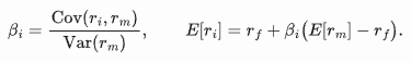
6.2 Security Market Line
Assets’ required returns depend solely on beta (βi), their sensitivity to market moves:

Python

# Calculate betas by regressing each asset on the market
import statsmodels.api as sm # For beta calculation via regression

print("\nCalculating Betas via Regression...")

betas_regression = {}

if not asset_returns.empty and not market_returns.empty and tickers:
    for t in tickers:
        if t in asset_returns.columns:
            df_regression = pd.concat([asset_returns[t], market_returns], axis=1).dropna()
            df_regression.columns = ['Asset', 'Market']
            if len(df_regression) > 1:
                X = sm.add_constant(df_regression['Market'])
                y = df_regression['Asset']
                try:
                    model = sm.OLS(y, X)
                    results = model.fit()
                    betas_regression[t] = results.params['Market']
                except Exception as e:
                    print(f"Could not calculate beta for {t} via regression: {e}")
                    betas_regression[t] = np.nan
            else:
                print(f"Not enough data points to calculate beta for {t} after alignment.")
                betas_regression[t] = np.nan
        else:
            print(f"Ticker {t} not found in asset_returns columns.")
            betas_regression[t] = np.nan
    print("Betas calculated via regression:", betas_regression)
else:
    print("Asset returns, market returns, or tickers list is empty. Skipping beta calculation.")

# Plot the Security Market Line (SML)
print("\nPlotting Security Market Line...")
if 'betas_regression' in locals() and betas_regression and \
   'market_returns' in locals() and not market_returns.empty and \
   'mean_daily_returns' in locals() and not mean_daily_returns.empty and \
   'tickers' in locals() and tickers and \
   'annual_trading_days' in locals():

    daily_risk_free_rate_sml = 0.0001 # Specific Rf for SML as per your code
    annual_risk_free_rate_sml = (1 + daily_risk_free_rate_sml)**annual_trading_days - 1
    
    market_mean_daily_sml = np.nan
    if isinstance(market_returns, pd.DataFrame):
        if market_returns.shape[1] == 0:
            market_mean_daily_sml = np.nan
            print("Warning: market_returns DataFrame is empty for SML. Market mean daily return is NaN.")
        elif market_returns.shape[1] == 1:
            market_mean_daily_sml = market_returns.iloc[:, 0].mean()
        else:
            market_mean_daily_sml = market_returns.iloc[:, 0].mean()
            print(f"Warning: market_returns DataFrame has {market_returns.shape[1]} columns for SML. Used mean of first column: {market_returns.columns[0]}.")
    elif isinstance(market_returns, pd.Series):
        market_mean_daily_sml = market_returns.mean()
    else:
        market_mean_daily_sml = np.nan
        print("Error: market_returns is of an unexpected type for SML. Market mean daily return set to NaN.")

    if pd.isna(market_mean_daily_sml):
        print("Market mean daily return is NaN for SML. Cannot plot SML accurately.")
    else:
        annual_market_return_sml = (1 + market_mean_daily_sml)**annual_trading_days - 1
        market_premium_sml = float(annual_market_return_sml - annual_risk_free_rate_sml)

        beta_values_sml = np.linspace(0, 2.5, 50)
        sml_expected_returns = annual_risk_free_rate_sml + beta_values_sml * market_premium_sml

        plt.figure(figsize=(10, 6))
        plt.plot(beta_values_sml, sml_expected_returns, 'r-', lw=2, label='Security Market Line (SML)')

        plotted_sml_assets_count = 0
        for t in tickers:
            if t in betas_regression and not pd.isna(betas_regression[t]) and \
               t in mean_daily_returns.index and not pd.isna(mean_daily_returns[t]):
                asset_beta = betas_regression[t]
                asset_historical_annual_return = (1 + mean_daily_returns[t])**annual_trading_days - 1
                plt.scatter(asset_beta, asset_historical_annual_return, s=70, label=f'{t} (Historical)')
                plt.text(asset_beta * 1.02, asset_historical_annual_return * 1.02, t, fontsize=9)
                plotted_sml_assets_count +=1
            else:
                print(f"Skipping {t} on SML plot: Beta or historical return missing/NaN.")
        
        if plotted_sml_assets_count == 0 and len(tickers) > 0 :
             print("Warning: No individual assets were plotted on the SML chart. Check beta/return data for all tickers.")

        plt.scatter(0, annual_risk_free_rate_sml, marker='s', s=100, color='blue', edgecolor='black', label='Risk-Free Asset ($R_f$)')
        plt.text(0 + 0.03, annual_risk_free_rate_sml, '$R_f$', fontsize=9)
        plt.scatter(1, annual_market_return_sml, marker='P', s=150, color='green', edgecolor='black', label='Market Portfolio ($\\beta=1$)')
        plt.text(1 * 1.02, annual_market_return_sml * 1.02, 'Market', fontsize=9)

        plt.title('Security Market Line (SML)')
        plt.xlabel('Beta ($\\beta$)')
        plt.ylabel('Annualized Expected Return ($E[R_i]$)')
        plt.legend()
        plt.grid(True)
        plt.axhline(0, color='black', lw=0.5)
        plt.axvline(0, color='black', lw=0.5)
        plt.show()
else:
    print("Prerequisite data for SML plot is missing or inconsistent. Skipping SML plot.")

Calculating Betas via Regression...
Betas calculated via regression: {'AAPL': np.float64(1.1896773359003732), 'MSFT': np.float64(1.1735182508973696), 'GOOG': np.float64(1.118838130001145)}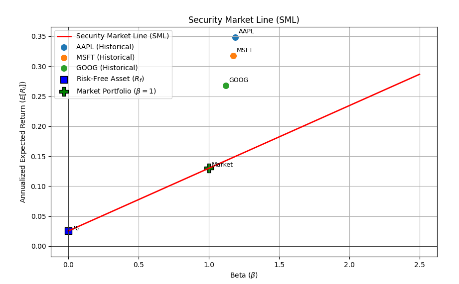

6.3 Beyond CAPM
Multi‑factor models (e.g., the Arbitrage Pricing Theory) express expected returns as a sum of exposures to several risk factors Fj:

with

With these tools — expected returns, risk measures, parameter estimation, portfolio optimization, market pricing of risk, and asset‑pricing models — you have a complete framework to quantify and manage the trade‑off between risk and return.