
In partnership with

Practical AI for Business Leaders

The AI Report is the #1 daily read for professionals who want to lead with AI, not get left behind.
You’ll get clear, jargon-free insights you can apply across your business—without needing to be technical.
400,000+ leaders are already subscribed.
👉 Join now and work smarter with AI.
🚀 Your Investing Journey Just Got Better: Premium Subscriptions Are Here! 🚀
It’s been 4 months since we launched our premium subscription plans at GuruFinance Insights, and the results have been phenomenal! Now, we’re making it even better for you to take your investing game to the next level. Whether you’re just starting out or you’re a seasoned trader, our updated plans are designed to give you the tools, insights, and support you need to succeed.
Here’s what you’ll get as a premium member:
Exclusive Trading Strategies: Unlock proven methods to maximize your returns.
In-Depth Research Analysis: Stay ahead with insights from the latest market trends.
Ad-Free Experience: Focus on what matters most—your investments.
Monthly AMA Sessions: Get your questions answered by top industry experts.
Coding Tutorials: Learn how to automate your trading strategies like a pro.
Masterclasses & One-on-One Consultations: Elevate your skills with personalized guidance.
Our three tailored plans—Starter Investor, Pro Trader, and Elite Investor—are designed to fit your unique needs and goals. Whether you’re looking for foundational tools or advanced strategies, we’ve got you covered.
Don’t wait any longer to transform your investment strategy. The last 4 months have shown just how powerful these tools can be—now it’s your turn to experience the difference.

The stock market is one of the most exciting and challenging domains to forecast. One powerful tool used in forecasting financial trends is Logistic Regression. But how exactly does it work, and can it really help in predicting stock market trends?
META Actual vs Predicted Movements
What is Logistic Regression?
Logistic regression is a statistical model commonly used for classification tasks.
Unlike linear regression, which predicts continuous values, logistic regression predicts probabilities that can be mapped to two categories, such as up or down in the context of stock prices.
It works by estimating the relationship between a dependent variable (in our case, the price movement) and one or more independent variables (like moving averages, volume, etc.).
The model then outputs probabilities, which can be converted into binary predictions: stock price will either go up or down.
Logistic regression is a great starting point for beginners in predictive modeling because it’s simple, interpretable, and requires less computational power compared to more complex models like neural networks.
Seeking impartial news? Meet 1440.
Every day, 3.5 million readers turn to 1440 for their factual news. We sift through 100+ sources to bring you a complete summary of politics, global events, business, and culture, all in a brief 5-minute email. Enjoy an impartial news experience.
How Does Logistic Regression Apply to Stock Market Forecasting?
Stock price movements are inherently volatile and influenced by various factors such as economic data, company performance, and market sentiment.
By using historical stock price data, we can build features such as moving averages, return percentages, and momentum indicators, and train a logistic regression model to predict price trends.
While logistic regression may not predict exact prices, it can help investors and traders make more informed decisions by identifying trends.
For instance, if the model predicts a high probability of an upward movement, investors may choose to buy, while a prediction of a downward movement may lead to selling or shorting the stock.
Pros
Simplicity and Interpretability: Logistic regression is easy to understand and implement. It provides clear output probabilities that can be interpreted and analyzed.
Speed: It’s computationally efficient, even with large datasets.
Good for Binary Outcomes: Since the stock market often involves predicting binary events (up or down), logistic regression is naturally suited for this task.
Works Well with Small Datasets: Unlike more complex models, logistic regression can perform well with smaller datasets, making it an excellent choice for stock forecasting when limited data is available.
Cons
Limited Flexibility: Logistic regression is linear. It can struggle to capture complex, non-linear relationships in data, which are common in financial markets.
Assumes Independence: It assumes that features are independent, which isn’t always the case in financial data where trends and signals may overlap.
Risk of Overfitting: With a large number of features, the model can overfit, meaning it performs well on the training data but poorly on new, unseen data.
Doesn’t Handle Sequential Data Well: Stock market data has a time-dependent nature (i.e., past prices affect future prices), and logistic regression doesn’t account for this temporal sequence very well.
Key Considerations
While logistic regression can be a great tool for stock market prediction, there are a few things to keep in mind:
Feature Engineering: The accuracy of the logistic regression model heavily depends on the features used. Technical indicators like moving averages, relative strength index (RSI), and volume changes can be useful for improving the model’s performance.
Data Quality: Financial markets are noisy, meaning the data can be volatile and unpredictable. Careful cleaning and processing of data are essential before applying any machine learning technique.
Model Evaluation: It’s important to evaluate the model using appropriate metrics such as accuracy, precision, recall, and confusion matrices to understand how well the model is performing.
The Role of Feature Engineering in Stock Market Forecasting
Feature engineering plays a critical role in improving the performance of machine learning models, including logistic regression. In stock market prediction, this could involve creating features like:
Moving Averages: Calculating the average closing price over a certain window (e.g., 5-day, 10-day) can help identify trends.
Price Returns: The percentage change in the price can be a good indicator of momentum.
Volatility Measures: Measures such as standard deviation can help capture market fluctuations.
Volume Data: Tracking the amount of stock being traded can indicate changes in investor sentiment.
By including these features, we can give the logistic regression model better insights into stock price behavior, potentially improving its ability to predict price movements.
A Python Example
Here is a python example on how you can experiment with Logistic Regression for forecasting a stock’s price.
All the code in this example can be found on this GitHub repository.
Setup the Environment
In your python environment, install the required libraries using the following command:
pip install pandas yfinance matplotlib datetime scikit-learn numpy seaborn tabulateOnce you have these installed, import them in your jupyter notebook:
import pandas as pd
import yfinance as yf
import matplotlib.pyplot as plt
from datetime import datetime
from sklearn.metrics import classification_report, confusion_matrix, accuracy_score
from sklearn.model_selection import train_test_split
from sklearn.linear_model import LogisticRegression
from sklearn.preprocessing import StandardScaler
from sklearn.pipeline import Pipeline
import seaborn as sns
from tabulate import tabulate
Download the Historical Data
Download the historical data to train the model, in this example we use META data from 2024-01-01 to the current date:
# Define the stock symbol and the date range for our data
stock_symbol = 'META'
start_date = '2020-01-01'
end_date = datetime.today().strftime('%Y-%m-%d')  # Sets end date to today's date
print(f"{stock_symbol}\nStart Date: {start_date}\nEnd Date: {end_date}")

df = yf.download(stock_symbol, start=start_date, end=end_date)

# Select the desired columns (first level of MultiIndex)
df.columns = df.columns.get_level_values(0)

# Keep only the columns you are interested in
df = df[['Close', 'Volume']]

# If the index already contains the dates, rename the index
df.index.name = 'Date'  # Ensure the index is named "Date"

# Resetting the index if necessary
df.reset_index(inplace=True)

# Ensure that the index is of type datetime
df['Date'] = pd.to_datetime(df['Date'])

# Set the 'Date' column as the index again (in case it's reset)
df.set_index('Date', inplace=True)

df.head()
Visualize Stock Chart
# Plot the original closing prices
plt.figure(figsize=(12, 6))

# Plot the 'Close' price column
plt.plot(df.index, df['Close'], label='Close Price', color='blue')

# Add title and labels
plt.title(f'{stock_symbol} - Closing Prices')
plt.xlabel('Date')
plt.ylabel('Price (USD)')

# Add a legend
plt.legend()

# Add gridlines
plt.grid(True)

plt.savefig(f'{stock_symbol}_closing_prices.png')

# Show the plot
plt.show()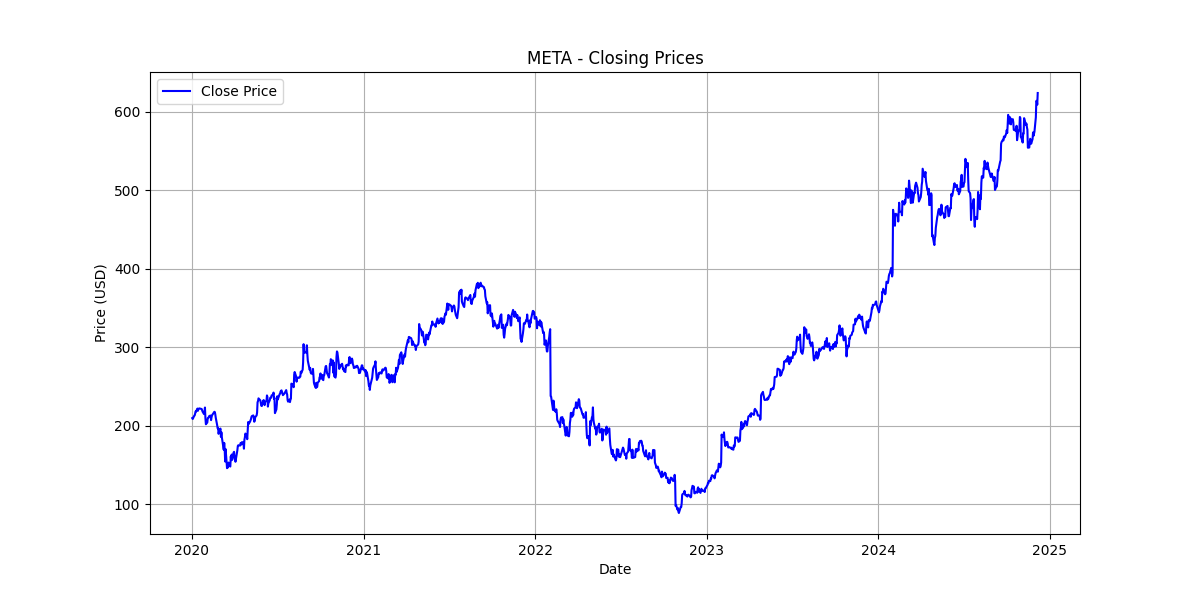
META Closing Price Chart
Target Variable
In this step, we create a Target column to indicate whether the stock price will go up or down in the next period.
A value of 1 represents that the price will go up, and 0 indicates a price drop.
We achieve this by comparing the next day’s closing price with the current day’s closing price.
# Add a column indicating whether the price will go up (1) or down (0)
df['Target'] = (df['Close'].shift(-1) > df['Close']).astype(int)

# Drop rows with NaN values (caused by shifting)
df.dropna(inplace=True)

# Display the head of the dataframe
df.head()
Feature Engineering
We now construct the features we need for training the model. I only highlight a few possible features, feel free to add your own features to improve the model.
Return Feature
This cell calculates the percentage change in the closing price (Return) to capture daily price movement.
# Add the 'Return' feature (percentage change)
df['Return'] = df['Close'].pct_change()

# Drop rows with NaN values after feature engineering
df.dropna(inplace=True)

# Display the head of the dataframe
df.head()
Weekday Feature
This cell adds a new feature called Weekday, which represents the day of the week as a numeric value (0 = Monday, 6 = Sunday). This feature helps capture any patterns or trends related to specific days of the week.
# Add 'Weekday' feature (numeric representation: 0=Monday, ..., 6=Sunday)
df['Weekday'] = df.index.dayofweek

# Display the head of the dataframe
df.head()
Relative Strength Index Feature
This cell calculates the Relative Strength Index (RSI), a momentum indicator that measures the speed and change of price movements.
The RSI helps identify overbought or oversold conditions in the market and is calculated using a 14-day window.
# Function to calculate Relative Strength Index (RSI)
def compute_rsi(data, window=14):
    delta = data.diff()  # Calculate the difference in price
    gain = (delta.where(delta > 0, 0)).rolling(window=window).mean()  # Positive gains
    loss = (-delta.where(delta < 0, 0)).rolling(window=window).mean()  # Negative losses
    rs = gain / loss  # Relative strength
    rsi = 100 - (100 / (1 + rs))  # RSI formula
    return rsi

# Add the 'RSI' feature
df['RSI'] = compute_rsi(df['Close'])

# Drop rows with NaN values after adding RSI
df.dropna(inplace=True)

# Display the head of the dataframe
df.head()
Volume Change Feature
This feature calculates the percentage change in volume from one day to the next. A positive value indicates an increase in volume, while a negative value suggests a decrease.
Tracking these changes can help identify significant shifts in market activity, which may precede price movements.
# Calculate the percentage change in volume (similar to how we calculate price change)
df['Volume_Change'] = df['Volume'].pct_change()

# Drop rows with NaN values (caused by percentage change)
df.dropna(inplace=True)

# Display the head of the dataframe
df.head()
Data Split
We split the data into training and testing sets, allocating 80% for training and 20% for testing. The split is reproducible due to the fixed random state and preserves the original data order by not shuffling which is necessary for time-series data.
# Define features and target variable
features = ['Return', 'Weekday', 'RSI', 'Volume_Change']

# Select features and target from the dataframe
X = df[features]
y = df['Target']

# Split data into training and testing sets
X_train, X_test, y_train, y_test = train_test_split(X, y, test_size=0.2, random_state=42, shuffle=False)
Train the Model
In this step, we create a pipeline to streamline the process of scaling the features and training the logistic regression model. The pipeline consists of two stages:
1. Scaling: The StandardScaler is used to standardize the features, ensuring they have a mean of 0 and a standard deviation of 1.
2. Model Training: A Logistic Regression model is used to learn from the scaled features.
The pipeline is then fitted on the training data (X_train, y_train), allowing the model to learn and make predictions based on the provided features.
# Create a pipeline for scaling and model training
model_pipeline = Pipeline([
    ('scaler', StandardScaler()),
    ('logreg', LogisticRegression())
])

# Fit the model
model_pipeline.fit(X_train, y_train)
Evaluate
Here, we make predictions using the trained model on both the training (X_train) and testing (X_test) data. The predictions are stored in y_train_pred and y_test_pred to be used for evaluation, respectively.
# Make predictions
y_train_pred = model_pipeline.predict(X_train)
y_test_pred = model_pipeline.predict(X_test)
This step calculates the confusion matrix for the training data, comparing the actual vs. predicted values.
The matrix is then visualized as a heatmap, where the colors represent the counts of true positives, true negatives, false positives, and false negatives.
This provides insight into the model’s performance in correctly classifying the target variable.
# Confusion matrix for training data
conf_matrix_train = confusion_matrix(y_train, y_train_pred)

# Plot Confusion Matrix Heatmap
plt.figure(figsize=(8, 6))
sns.heatmap(conf_matrix_train, annot=True, fmt="d", cmap="Greens", xticklabels=['Down (0)', 'Up (1)'], yticklabels=['Down (0)', 'Up (1)'])
plt.title("Confusion Matrix (Training Data)")
plt.xlabel("Predicted")
plt.ylabel("Actual")
plt.show()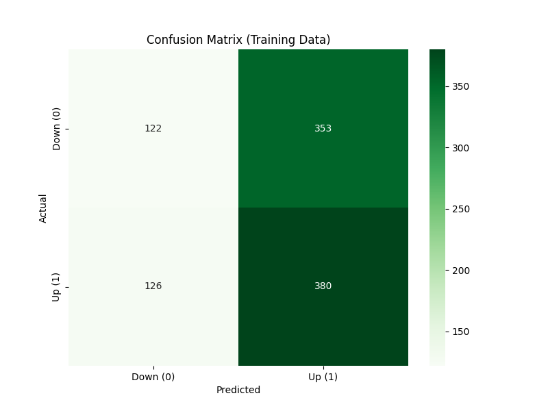
Training Data Confusion Matrix
Training Data Results
# Generate the classification report
train_report = classification_report(y_train, y_train_pred, output_dict=True)

# Format the report for display using tabulate
report_table = []
for label, metrics in train_report.items():
    if isinstance(metrics, dict):  # For the metrics of each class
        row = [label] + [f"{metrics['precision']:.3f}", f"{metrics['recall']:.3f}", f"{metrics['f1-score']:.3f}", f"{metrics['support']}"]
    else:  # For accuracy, macro avg, and weighted avg
        row = [label] + [f"{metrics:.3f}" if isinstance(metrics, float) else metrics]
    report_table.append(row)

# Print the table in a clean format
print("Training Performance:")
print(tabulate(report_table, headers=["Metric", "Precision", "Recall", "F1-Score", "Support"], tablefmt="pretty"))
Training Performance:
+--------------+-----------+--------+----------+---------+
| Metric | Precision | Recall | F1-Score | Support |
+--------------+-----------+--------+----------+---------+
| 0 | 0.492 | 0.257 | 0.337 | 475.0 |
| 1 | 0.518 | 0.751 | 0.613 | 506.0 |
| accuracy | 0.512 | | | |
| macro avg | 0.505 | 0.504 | 0.475 | 981.0 |
| weighted avg | 0.506 | 0.512 | 0.480 | 981.0 |
+--------------+-----------+--------+----------+---------+Testing Data Results
# Generate the classification report
test_report = classification_report(y_test, y_test_pred, output_dict=True)

# Format the report for display using tabulate
report_table = []
for label, metrics in test_report.items():
    if isinstance(metrics, dict):  # For the metrics of each class
        row = [label] + [f"{metrics['precision']:.3f}", f"{metrics['recall']:.3f}", f"{metrics['f1-score']:.3f}", f"{metrics['support']}"]
    else:  # For accuracy, macro avg, and weighted avg
        row = [label] + [f"{metrics:.3f}" if isinstance(metrics, float) else metrics]
    report_table.append(row)

# Print the table in a clean format
print("Testing Performance:")
print(tabulate(report_table, headers=["Metric", "Precision", "Recall", "F1-Score", "Support"], tablefmt="pretty"))
Testing Performance:
+--------------+-----------+--------+----------+---------+
| Metric | Precision | Recall | F1-Score | Support |
+--------------+-----------+--------+----------+---------+
| 0 | 0.582 | 0.411 | 0.482 | 112.0 |
| 1 | 0.605 | 0.754 | 0.671 | 134.0 |
| accuracy | 0.598 | | | |
| macro avg | 0.594 | 0.582 | 0.576 | 246.0 |
| weighted avg | 0.595 | 0.598 | 0.585 | 246.0 |
+--------------+-----------+--------+----------+---------+Accuracy Scores
# Accuracy score
train_accuracy = accuracy_score(y_train, y_train_pred)
test_accuracy = accuracy_score(y_test, y_test_pred)
print(f"Training Accuracy: {train_accuracy:.2f}")
print(f"Testing Accuracy: {test_accuracy:.2f}")
Training Accuracy: 0.51
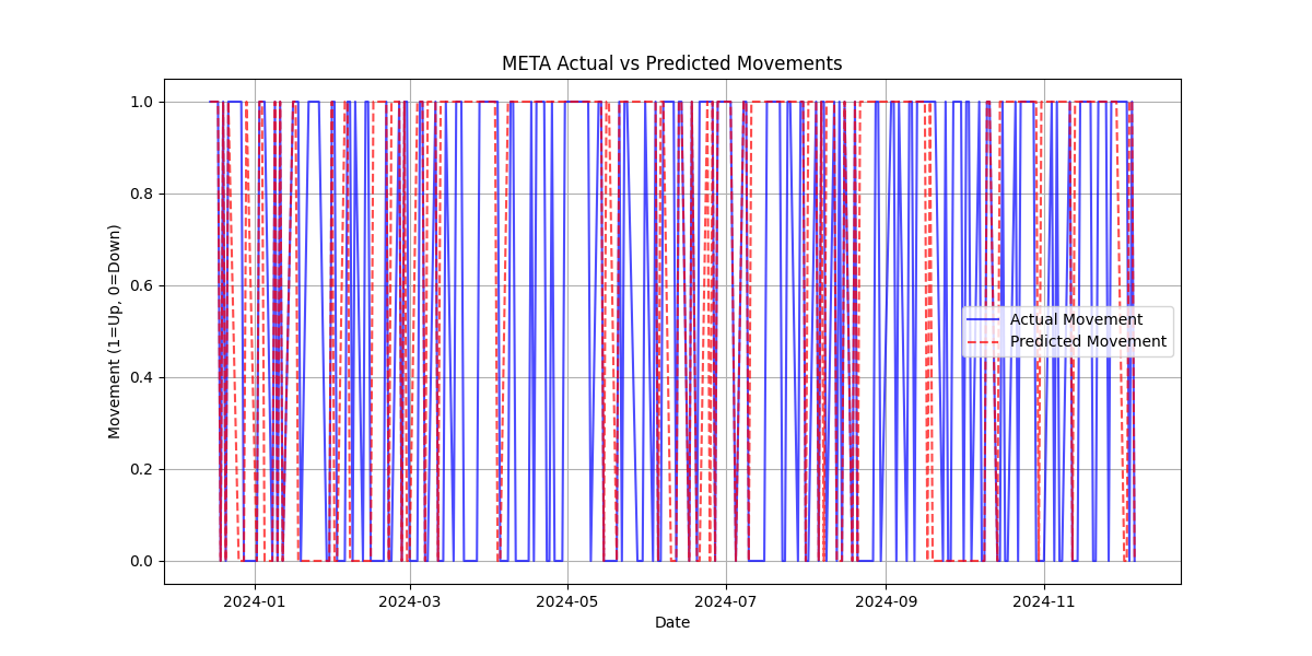
Testing Accuracy: 0.60Visualizing Actual vs Predicted Movements
In this step, we add the predictions made by the model to the test dataset and plot the actual vs predicted movements.
The actual stock price movement (up or down) is compared with the predicted movement, allowing us to visually assess how well the model is performing over time.
By plotting both the actual and predicted movements on the same graph, we can identify trends and evaluate the accuracy of the model’s predictions.
This visualization helps to better understand how the model is tracking market movements and highlights any discrepancies between predicted and actual outcomes.
# Add predictions to the test set for plotting
X_test['Predicted'] = y_test_pred
X_test['Actual'] = y_test.values

plt.figure(figsize=(12, 6))

# Plot actual vs predicted
plt.plot(X_test.index, X_test['Actual'], label='Actual Movement', color='blue', alpha=0.7)
plt.plot(X_test.index, X_test['Predicted'], label='Predicted Movement', color='red', linestyle='--', alpha=0.7)

plt.title(f'{stock_symbol} Actual vs Predicted Movements')
plt.xlabel('Date')
plt.ylabel('Movement (1=Up, 0=Down)')
plt.legend()
plt.grid(True)

plt.savefig(f'{stock_symbol}_movement_forecast.png')
plt.show()
Actual vs Predicted Movements
Conclusion
Logistic regression is a simple yet effective model for stock market forecasting, especially for binary predictions like up or down.
While it has its limitations, such as its inability to handle non-linear relationships and sequential data, it still offers a valuable approach for building predictive models, especially when coupled with good feature engineering.
By understanding the pros, cons, and key considerations, you can decide whether logistic regression is the right tool for your stock market forecasting needs.