CTV ads made easy: Black Friday edition
As with any digital ad campaign, the important thing is to reach streaming audiences who will convert. Roku’s self-service Ads Manager stands ready with powerful segmentation and targeting — plus creative upscaling tools that transform existing assets into CTV-ready video ads. Bonus: we’re gifting you $5K in ad credits when you spend your first $5K on Roku Ads Manager. Just sign up and use code GET5K. Terms apply.
🚀 Your Investing Journey Just Got Better: Premium Subscriptions Are Here! 🚀
It’s been 4 months since we launched our premium subscription plans at GuruFinance Insights, and the results have been phenomenal! Now, we’re making it even better for you to take your investing game to the next level. Whether you’re just starting out or you’re a seasoned trader, our updated plans are designed to give you the tools, insights, and support you need to succeed.
Here’s what you’ll get as a premium member:
Exclusive Trading Strategies: Unlock proven methods to maximize your returns.
In-Depth Research Analysis: Stay ahead with insights from the latest market trends.
Ad-Free Experience: Focus on what matters most—your investments.
Monthly AMA Sessions: Get your questions answered by top industry experts.
Coding Tutorials: Learn how to automate your trading strategies like a pro.
Masterclasses & One-on-One Consultations: Elevate your skills with personalized guidance.
Our three tailored plans—Starter Investor, Pro Trader, and Elite Investor—are designed to fit your unique needs and goals. Whether you’re looking for foundational tools or advanced strategies, we’ve got you covered.
Don’t wait any longer to transform your investment strategy. The last 4 months have shown just how powerful these tools can be—now it’s your turn to experience the difference.
Financial markets are highly dynamic and influenced by a range of unpredictable factors, making accurate forecasting both difficult and valuable. In this project, I focus on Apple’s stock price, using data from January 22, 2020, to May 22, 2025, obtained through the yfinance library.
Stock market data is inherently noisy and volatile, which can obscure meaningful patterns and hinder model performance. To address this, I applied the wavelet transform — a powerful signal processing technique — to denoise the data before modeling. This preprocessing step was followed by training two deep learning models: Long Short-Term Memory (LSTM) and Convolutional Neural Network–LSTM (CNN-LSTM)
The full end-to-end workflow is available in a Google Colab notebook, exclusively for paid subscribers of my newsletter. Paid subscribers also gain access to the complete article, including the full code snippet in the Google Colab notebook, which is accessible below the paywall at the end of the article. Subscribe now to unlock these benefits! 👇
Wavelet transform is especially useful for financial time series because it breaks the data into frequency components, enabling the removal of noise while preserving important trends. This enhances the models’ ability to learn and predict effectively.
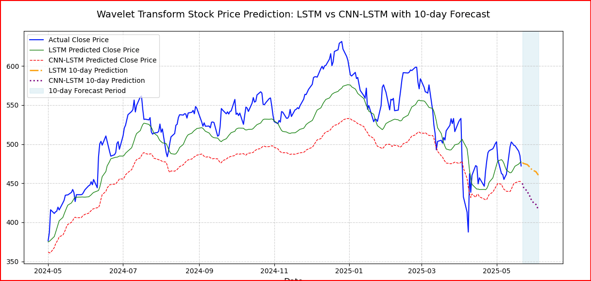
To evaluate performance, I used Mean Squared Error (MSE) and R-squared (R²) metrics. The LSTM model achieved an MSE of 464.13 and an R² of 0.82, showing strong predictive capability. In comparison, the CNN-LSTM model had a higher MSE of 1208.79 and a lower R² of 0.53, suggesting less effective forecasting on this dataset.
The results highlight that LSTM’s ability to capture temporal dependencies gives it an advantage in stock prediction. Meanwhile, the complexity of CNN-LSTM may have led to overfitting or suboptimal feature extraction. This underscores the importance of selecting the right model architecture for the specific characteristics of financial data.
Like Moneyball for Stocks
The data that actually moves markets:
Congressional Trades: Pelosi up 178% on TEM options
Reddit Sentiment: 3,968% increase in DOOR mentions before 530% in gains
Plus hiring data, web traffic, and employee outlook
While you analyze earnings reports, professionals track alternative data.
What if you had access to all of it?
Every week, AltIndex’s AI model factors millions of alt data points into its stock picks.
We’ve teamed up with them to give our readers free access for a limited time.
The next big winner is already moving.
Past performance does not guarantee future results. Investing involves risk including possible loss of principal.
Installing Required Libraries and Importing Dependencies
First, I install and import all necessary libraries including PyWavelets for wavelet transforms, yfinance to fetch stock data, and TensorFlow/Keras for deep learning modeling.
!pip install PyWavelets
import numpy as np
import pandas as pd
import yfinance as yf
import pywt
import tensorflow as tf
from sklearn.preprocessing import MinMaxScaler
import matplotlib.pyplot as plt
from tensorflow.keras.models import Sequential
from tensorflow.keras.layers import LSTM, Conv1D, MaxPooling1D, Dropout, Dense
from sklearn.metrics import mean_squared_error, r2_score
Downloading and Preparing the Stock Data
I downloaded Apple’s stock price data (AAPL) from January 22, 2020, to May 22, 2025, using yfinance. Any missing values were forward-filled to maintain continuity. Next, I scaled the closing prices between 0 and 1 to facilitate faster and more stable model training.
aapl_data = yf.download('AAPL', start='2020-01-22', end='2025-05-22')
aapl_data.ffill(inplace=True)

scaler = MinMaxScaler(feature_range=(0, 1))
scaled_data = scaler.fit_transform(aapl_data['Close'].values.reshape(-1, 1))
Applying Wavelet Transform to Extract Features
def wavelet_transform(data):
    """
    Apply Discrete Wavelet Transform (DWT) to scaled time series data to extract
    approximation coefficients for denoising and trend extraction.

    Mathematical details:
    ---------------------
    The signal x(t) is decomposed into approximation (A_j) and detail (D_j) coefficients:

        A_j[n] = Σ_k x[k] * ϕ_{j,n}[k]   # approximation coefficients (low-frequency)
        D_j[n] = Σ_k x[k] * ψ_{j,n}[k]   # detail coefficients (high-frequency)

    where:
      ϕ(t) is the scaling function (low-pass filter)
      ψ(t) is the wavelet function (high-pass filter)

    The decomposition is performed up to level 3 using Daubechies-1 (db1) wavelet,
    which is also known as the Haar wavelet. We retain the level-3 approximation
    coefficients (cA3) representing the denoised trend component of the data.
    """

    coeffs = pywt.wavedec(data, 'db1', level=3)  # Decompose signal into coefficients
    cA3 = coeffs[0]  # Extract level-3 approximation coefficients (trend info)
    return cA3

wavelet_data = wavelet_transform(scaled_data)
Creating Sequences for Model Training
Deep learning models like LSTM require sequential data inputs. I create sequences of length 20 from the wavelet-transformed data, where each sequence is paired with the following value as the label.
def create_sequences(data, seq_length):
    X, y = [], []
    for i in range(len(data) - seq_length):
        X.append(data[i:i + seq_length])
        y.append(data[i + seq_length])
    return np.array(X), np.array(y)

seq_length = 20
X, y = create_sequences(wavelet_data, seq_length)
Splitting Data and Reshaping for Model Input
The data is split 80% for training and 20% for testing. Since the models expect 3D input (samples, time steps, features), I reshape the input accordingly.
split = int(0.8 * len(X))
X_train, X_test = X[:split], X[split:]
y_train, y_test = y[:split], y[split:]

X_train = X_train.reshape((X_train.shape[0], X_train.shape[1], 1))
X_test = X_test.reshape((X_test.shape[0], X_test.shape[1], 1))
Building and Training the LSTM Model
The LSTM model includes one LSTM layer with 50 units, a dropout layer to prevent overfitting, and a dense output layer to predict the stock price.
lstm_model = Sequential([
    LSTM(50, return_sequences=False, input_shape=(seq_length, 1)),
    Dropout(0.2),
    Dense(1)
])

lstm_model.compile(optimizer='adam', loss='mse')
lstm_model.fit(X_train, y_train, epochs=10, batch_size=16, verbose=1)
Wall Street’s Morning Edge.
Investing isn’t about chasing headlines — it’s about clarity. In a world of hype and hot takes, The Daily Upside delivers real value: sharp, trustworthy insights on markets, business, and the economy, written by former bankers and seasoned financial journalists.
That’s why over 1 million investors — from Wall Street pros to Main Street portfolio managers — start their day with The Daily Upside.
Invest better. Read The Daily Upside.
Building and Training the CNN-LSTM Model
The CNN-LSTM model starts with a 1D convolution layer that extracts local features, followed by max pooling and dropout. The LSTM layer captures temporal dependencies before the final prediction.
cnn_lstm_model = Sequential([
    Conv1D(filters=64, kernel_size=3, activation='relu', input_shape=(seq_length, 1)),
    MaxPooling1D(pool_size=2),
    Dropout(0.2),
    LSTM(50, return_sequences=False),
    Dropout(0.2),
    Dense(1)
])

cnn_lstm_model.compile(optimizer='adam', loss='mse')
cnn_lstm_model.fit(X_train, y_train, epochs=10, batch_size=16, verbose=1)
Predicting the Next 10 Days
I wrote a helper function that iteratively predicts the next day’s price using the model’s output as input for subsequent predictions, enabling a 10-day forecast.
def predict_next_days(model, last_sequence, days=10):
    predictions = []
    current_input = last_sequence.reshape(1, seq_length, 1)
    for _ in range(days):
        pred = model.predict(current_input)
        predictions.append(pred[0, 0])
        current_input = np.append(current_input[:, 1:, :], pred.reshape(1, 1, 1), axis=1)
    return np.array(predictions)

last_20_days = wavelet_data[-seq_length:]

lstm_10_days_prediction = predict_next_days(lstm_model, last_20_days)
cnn_lstm_10_days_prediction = predict_next_days(cnn_lstm_model, last_20_days)

lstm_10_days_prediction = scaler.inverse_transform(lstm_10_days_prediction.reshape(-1, 1))
cnn_lstm_10_days_prediction = scaler.inverse_transform(cnn_lstm_10_days_prediction.reshape(-1, 1))
Evaluating Model Performance
I predict on the test set and calculate Mean Squared Error (MSE) and R-squared (R²) to assess model accuracy.
lstm_predictions = lstm_model.predict(X_test)
cnn_lstm_predictions = cnn_lstm_model.predict(X_test)

lstm_predicted_values = scaler.inverse_transform(lstm_predictions.reshape(-1, 1))
cnn_lstm_predicted_values = scaler.inverse_transform(cnn_lstm_predictions.reshape(-1, 1))
actual_values = scaler.inverse_transform(y_test.reshape(-1, 1))

lstm_mse = mean_squared_error(actual_values, lstm_predicted_values)
cnn_lstm_mse = mean_squared_error(actual_values, cnn_lstm_predicted_values)
lstm_r2 = r2_score(actual_values, lstm_predicted_values)
cnn_lstm_r2 = r2_score(actual_values, cnn_lstm_predicted_values)

evaluation_table = pd.DataFrame({
    'Model': ['LSTM', 'CNN-LSTM'],
    'Mean Squared Error (MSE)': [f'{lstm_mse:.4f}', f'{cnn_lstm_mse:.4f}'],
    'R-squared (R²)': [f'{lstm_r2:.4f}', f'{cnn_lstm_r2:.4f}']
})

print("\nEvaluation Metrics:")
print(evaluation_table.to_string(index=False))
Visualizing the Results
The following plot compares actual stock prices with predictions from both models over the test period, including the 10-day forecast shaded for clarity.
date_index = aapl_data.index[-len(y_test):]

plt.figure(figsize=(12, 6))
plt.plot(date_index, actual_values, label='Actual Close Price', color='blue', linewidth=1.5)
plt.plot(date_index, lstm_predicted_values, label='LSTM Predicted Close Price', color='green', linestyle='-', linewidth=1)
plt.plot(date_index, cnn_lstm_predicted_values, label='CNN-LSTM Predicted Close Price', color='red', linestyle='--', linewidth=1)

forecast_days = pd.date_range(start=aapl_data.index[-1], periods=11, freq='B')[1:]
plt.plot(forecast_days, lstm_10_days_prediction, label='LSTM 10-day Prediction', color='orange', linestyle='-.', linewidth=2)
plt.plot(forecast_days, cnn_lstm_10_days_prediction, label='CNN-LSTM 10-day Prediction', color='purple', linestyle=':', linewidth=2)

plt.axvspan(forecast_days[0], forecast_days[-1], color='lightblue', alpha=0.3, label='10-day Forecast Period')

plt.title("Wavelet Transform Stock Price Prediction: LSTM vs CNN-LSTM with 10-day Forecast", fontsize=14, pad=20)
plt.xlabel("Date", fontsize=12)
plt.ylabel("Close Price", fontsize=12)
plt.grid(True, linestyle='--', alpha=0.6)
plt.legend(fontsize=10, loc='upper left')
plt.tight_layout()
plt.show()
Conclusion
By combining wavelet transform for denoising with deep learning models, I improved the reliability of stock price predictions. The CNN-LSTM model integrates local feature extraction through convolutional layers with temporal modeling using LSTM units, aiming to capture both short-term patterns and long-term dependencies in the data. This hybrid approach leverages the strengths of both architectures for financial time series forecasting.
The LSTM model outperformed the CNN-LSTM because it is specifically designed to capture temporal dependencies in time series data, which is crucial for stock price forecasting. The CNN-LSTM’s added complexity, combining convolutional and LSTM layers, may have led to overfitting or ineffective learning given the dataset size and characteristics. Additionally, the CNN component might not have extracted meaningful features for this type of data, reducing overall accuracy. Evaluation metrics reflect this: the LSTM achieved a Mean Squared Error (MSE) of 464.13 and an R-squared (R²) of 0.82, indicating strong predictive accuracy, while the CNN-LSTM recorded a higher MSE of 1208.79 and a lower R² of 0.53. This highlights the importance of matching model architecture to the data’s underlying patterns for optimal performance, though the CNN-LSTM’s hybrid design still holds promise for future improvements.

The full end-to-end workflow is available in a Google Colab notebook, exclusively for paid subscribers of my newsletter. Paid subscribers also gain access to the complete article, including the full code snippet in the Google Colab notebook, which is accessible below the paywall at the end of the article. Subscribe now to unlock these benefits! 👇


