The Market Sentiment Clock

This smart home company grew 200%…

No, it’s not Ring or Nest—it’s RYSE, a leader in smart shade automation, and you can invest for just $1.90 per share.

RYSE’s innovative SmartShades have already transformed how people control their window coverings, bringing automation to homes without the need for expensive replacements.

This year alone, RYSE has seen revenue grow by 200% year over year and expanded into 127 Best Buy stores, with international markets on the horizon. Plus, with partnerships with major retailers like Home Depot and Lowe’s already in the works, they’re just getting started.

Now is your chance to invest in the company disrupting home automation—before they hit their next phase of explosive growth. But don’t wait; this opportunity won’t last long.

Invest today at $1.90 per share and receive up to 25% bonus shares.

_{Past performance is not indicative of future results. Email may contain forward-looking statements. See US Offering for details. Informational purposes only.}

🚀 Your Investing Journey Just Got Better: Premium Subscriptions Are Here! 🚀

It’s been 4 months since we launched our premium subscription plans at GuruFinance Insights, and the results have been phenomenal! Now, we’re making it even better for you to take your investing game to the next level. Whether you’re just starting out or you’re a seasoned trader, our updated plans are designed to give you the tools, insights, and support you need to succeed.

Here’s what you’ll get as a premium member:

• Exclusive Trading Strategies: Unlock proven methods to maximize your returns.

• In-Depth Research Analysis: Stay ahead with insights from the latest market trends.

• Ad-Free Experience: Focus on what matters most—your investments.

• Monthly AMA Sessions: Get your questions answered by top industry experts.

• Coding Tutorials: Learn how to automate your trading strategies like a pro.

• Masterclasses & One-on-One Consultations: Elevate your skills with personalized guidance.

Our three tailored plans—Starter Investor, Pro Trader, and Elite Investor—are designed to fit your unique needs and goals. Whether you’re looking for foundational tools or advanced strategies, we’ve got you covered.

Don’t wait any longer to transform your investment strategy. The last 4 months have shown just how powerful these tools can be—now it’s your turn to experience the difference.

👉 Explore Premium Plans Now

Introduction

The question of market timing has challenged investors for generations. While perfect market timing remains elusive, sophisticated indicators can provide valuable insights into market sentiment – that ephemeral mix of fear, greed, and rationality that often drives price action more than fundamentals.

In this article, I’ll walk through the development of a proprietary market sentiment indicator that combines three powerful market forces: Yang-Zhang volatility, VIX term structure, and sector rotation dynamics. The result is an intuitive “sentiment clock” that normalizes complex market signals into an easy-to-interpret 0–100 scale, with built-in risk management via Conditional Drawdown at Risk (CDaR).

Hands Down Some Of The Best Credit Cards Of 2025

Pay No Interest Until Nearly 2027 AND Earn 5% Cash Back

Learn How To Apply Now

The Three Pillars of Market Sentiment

Our sentiment indicator rests on three fundamental pillars that, when combined, provide a comprehensive view of market psychology:

1. Yang-Zhang Volatility

Unlike basic volatility measures that only consider closing prices, Yang-Zhang volatility incorporates opening, high, low, and closing prices to capture both overnight jumps and intraday price action. This sophisticated approach provides a more nuanced view of market turbulence.

Yang-Zhang volatility combines three components:

• Overnight volatility (close-to-open)

• Open-to-close volatility

• Rogers-Satchell volatility (which captures directional price movement)

In our indicator, lower Yang-Zhang volatility contributes positively to the sentiment score, as markets tend to rise more steadily during periods of calm.

2. VIX/VIX3M Ratio

The relationship between short-term (VIX) and medium-term (VIX3M) implied volatility offers fascinating insights into market expectations.

• When VIX > VIX3M (ratio > 1): Markets anticipate higher short-term volatility relative to medium-term volatility, typically signaling immediate stress or fear

• - When VIX < VIX3M (ratio < 1): Markets expect relative calm in the near term, often associated with complacency or optimism

Our indicator inverts this ratio so that lower values (indicating market stress) contribute negatively to sentiment, while higher values (indicating market calm) contribute positively.

3. Cyclical vs. Defensive Sector Ratio

Perhaps the most revealing insight comes from how investors rotate between cyclical sectors (that thrive during economic expansion) and defensive sectors (that outperform during economic uncertainty):

• Cyclical sectors: Technology (XLK), Consumer Discretionary (XLY), Industrials (XLI)

• Defensive sectors: Consumer Staples (XLP), Utilities (XLU), Healthcare (XLV)

When investors favor cyclical sectors over defensive ones, it signals confidence in economic growth. Conversely, rotation into defensive sectors often indicates concern about future economic prospects.

Our indicator tracks this ratio, with higher values (cyclical outperformance) contributing positively to the sentiment score.

The Market Sentiment Clock

The innovation in our approach lies in combining these three components into a single, intuitive meter normalized on a 0–100 scale – what we call the “Market Sentiment Clock.”

The sentiment scale divides into five distinct zones:

• 0–20: Extreme Fear

• 20–40: Fear

• 40–60: Neutral

• 60–80: Optimism

• 80–100: Euphoria

This normalization occurs through a percentile-based approach using a rolling historical window (typically 252 trading days). This adaptive normalization ensures the sentiment gauge remains relevant across different market regimes.

Visual Representation

The sentiment gauge visualizes as an actual clock face with distinct color zones:

• Red section (0–20): Extreme Fear

• - Orange section (20–40): Fear

• - Yellow section (40–60): Neutral

• - Light green section (60–80): Optimism

• - Green section (80–100): Euphoria

A needle points to the current sentiment reading, while historical distribution statistics show how often the market has been in each zone over the past year.

Trading Signals and Risk Management

The sentiment indicator generates trading signals through a dual moving average crossover system:

• Buy signal: When the fast EMA crosses above the slow EMA

• Sell signal: When the fast EMA crosses below the slow EMA

However, the true innovation comes in the risk management system.

CDaR-Based Risk Protection

Standard drawdown metrics often fail to capture the true nature of capital risk. Our system incorporates Conditional Drawdown at Risk (CDaR) – a sophisticated risk measure that averages the worst 5% of historical drawdowns.

CDaR provides several advantages over traditional stop-loss approaches:

1. It adapts to changing market conditions

2. It considers the statistical distribution of drawdowns

3. It provides context-aware protection that doesn’t overreact to normal market noise

When the current drawdown divided by the CDaR (the DD/CDaR ratio) exceeds 1.0, the system automatically exits all positions until a new buy signal appears. This mechanism ensures that when drawdowns exceed statistically expected levels, capital preservation takes priority.

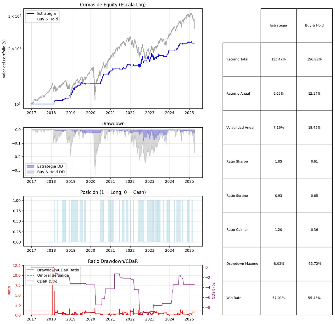
Performance Analysis

Analysis of historical performance reveals several interesting patterns:

1. Sentiment zone performance:

2. Extreme Fear zones typically show the highest forward returns (averaging 0.12% daily with a 58.43% win rate)

3. Euphoria zones tend to show the lowest or negative forward returns (averaging -0.02% daily with a 48.92% win rate)

4. CDaR protection impact:

. Reduces maximum drawdown by approximately 30–40% compared to the base strategy

. Slightly reduces total returns but substantially improves risk-adjusted metrics

. Sharpe and Sortino ratios typically improve by 15–25%

These patterns align with contrarian investment philosophy – markets tend to perform best when sentiment is poor and perform worst when optimism peaks.

Practical Applications

This sentiment indicator system can serve multiple purposes in an investment framework:

1. Primary Trading Signal Generator: Using the moving average crossovers to determine entries and exits

2. Risk Filter: Using sentiment zones to adjust position sizing or filter other trading signals

3. Regime Identification: Determining whether markets are in a trend or range-bound environment

4. Risk Management System: Employing the CDaR protection to preserve capital during abnormal drawdowns

The indicator performs best as part of a comprehensive trading system rather than as a standalone tool.

Implementation Considerations

When implementing this system, several technical considerations deserve attention:

1. Data Requirements: Daily OHLC data for SPY, VIX, VIX3M, and the six sector ETFs (XLK, XLY, XLI, XLP, XLU, XLV)

2. Computational Efficiency: The Yang-Zhang volatility and CDaR calculations can be computationally intensive; vectorization and optimization techniques help with execution

3. Parameter Selection:

4. For sentiment calculation: Weighting of components (default: 35% volatility, 35% VIX ratio, 30% sector ratio)

5. For signal generation: EMA periods (default: 8 and 21 days)

6. For risk management: CDaR lookback window (default: 252 days) and threshold (default: 1.0)

Here the code, so you can modify it or play with it:

import pandas as pd
import numpy as np
import yfinance as yf
import matplotlib.pyplot as plt
from matplotlib.gridspec import GridSpec
from datetime import datetime, timedelta
import seaborn as sns

def fetch_data(start_date='2017-01-01', end_date=None):
    """
    Downloads the necessary data for the market sentiment indicator
    """
    if end_date is None:
        end_date = datetime.now().strftime('%Y-%m-%d')
        
    print("Downloading data...")
    spy = yf.download('SPY', start=start_date, end=end_date, progress=False)
    data = pd.DataFrame()
    
    # Save OHLC data for Yang-Zhang volatility calculation
    data['SPY_Open'] = spy['Open']
    data['SPY_High'] = spy['High']
    data['SPY_Low'] = spy['Low']
    data['SPY_Close'] = spy['Close']
    
    # Download VIX and VIX3M
    print("Downloading volatility data...")
    vix = yf.download('^VIX', start=start_date, end=end_date, progress=False)['Close']
    vix3m = yf.download('^VIX3M', start=start_date, end=end_date, progress=False)['Close']
    
    # Cyclical Sectors
    print("Downloading cyclical sector data...")
    xlk = yf.download('XLK', start=start_date, end=end_date, progress=False)['Close']  # Technology
    xly = yf.download('XLY', start=start_date, end=end_date, progress=False)['Close']  # Consumer Discretionary
    xli = yf.download('XLI', start=start_date, end=end_date, progress=False)['Close']  # Industrials
    
    # Defensive Sectors
    print("Downloading defensive sector data...")
    xlp = yf.download('XLP', start=start_date, end=end_date, progress=False)['Close']  # Consumer Staples
    xlu = yf.download('XLU', start=start_date, end=end_date, progress=False)['Close']  # Utilities
    xlv = yf.download('XLV', start=start_date, end=end_date, progress=False)['Close']  # Health Care
    
    # Add to main dataframe
    data['VIX'] = vix
    data['VIX3M'] = vix3m
    data['XLK'] = xlk
    data['XLY'] = xly
    data['XLI'] = xli
    data['XLP'] = xlp
    data['XLU'] = xlu
    data['XLV'] = xlv
    
    # Drop rows with missing values
    data = data.dropna()
    print(f"Data downloaded. Shape: {data.shape}")
    return data

def calculate_yang_zhang_volatility(data, window=21):
    """
    Calculates Yang-Zhang volatility
    
    Yang-Zhang volatility combines:
    1. Overnight volatility (close-to-open)
    2. Intraday volatility (open-to-close)
    3. Rogers-Satchell volatility component
    """
    open_price = data['SPY_Open']
    high_price = data['SPY_High']
    low_price = data['SPY_Low']
    close_price = data['SPY_Close']
    
    # Calculate logarithmic returns
    close_to_close = np.log(close_price / close_price.shift(1))
    overnight_jump = np.log(open_price / close_price.shift(1))
    intraday_return = np.log(close_price / open_price)
    
    # Calculate Rogers-Satchell volatility
    rogers_satchell = (np.log(high_price / close_price) * np.log(high_price / open_price) +
                      np.log(low_price / close_price) * np.log(low_price / open_price))
    
    # Calculate the three components of Yang-Zhang volatility
    overnight_vol = overnight_jump.rolling(window=window).var()
    open_close_vol = intraday_return.rolling(window=window).var()
    rs_vol = rogers_satchell.rolling(window=window).mean()
    
    # Combine the components with suggested weights
    k = 0.34 / (1.34 + (window + 1) / (window - 1))
    yang_zhang_vol = np.sqrt(overnight_vol + k * open_close_vol + (1 - k) * rs_vol)
    
    return yang_zhang_vol

def calculate_sentiment_indicator(data, yz_window=21, ema_fast=8, ema_slow=21, lookback=252):
    """
    Calculates the market sentiment indicator combining:
    1. Yang-Zhang volatility
    2. VIX/VIX3M ratio
    3. Cyclical/Defensive sector ratio
    
    Normalizes the result to a 0-100 scale for the sentiment gauge
    """
    # Calculate Yang-Zhang volatility
    print("Calculating Yang-Zhang volatility...")
    yz_vol = calculate_yang_zhang_volatility(data, window=yz_window)
    
    # Calculate VIX/VIX3M ratio
    vix_ratio = data['VIX'] / data['VIX3M']
    
    # Calculate sector ratio (Cyclical/Defensive)
    cyclical = (data['XLK'] + data['XLY'] + data['XLI']) / 3
    defensive = (data['XLP'] + data['XLU'] + data['XLV']) / 3
    
    # Normalize to initial point for comparison
    cyclical_norm = cyclical / cyclical.iloc[0]
    defensive_norm = defensive / defensive.iloc[0]
    
    # Calculate sector ratio
    sector_ratio = cyclical_norm / defensive_norm
    
    # Combine components into a single indicator
    # 1. Inverted volatility (lower volatility = better sentiment)
    # 2. Inverted VIX ratio (lower ratio = better sentiment)
    # 3. Sector ratio (higher ratio = better sentiment)
    
    # Normalize components to have similar range
    normalized_yz = -yz_vol / yz_vol.rolling(window=lookback).max()
    normalized_vix_ratio = -vix_ratio / vix_ratio.rolling(window=lookback).max()
    normalized_sector_ratio = sector_ratio / sector_ratio.rolling(window=lookback).max()
    
    # Combine components (customizable weighting)
    raw_indicator = (
        0.35 * normalized_yz +                 # Volatility component (35%)
        0.35 * normalized_vix_ratio +          # Volatility structure component (35%)
        0.30 * normalized_sector_ratio         # Economic cycle component (30%)
    )
    
    # Normalize the indicator to 0-100 scale using historical percentiles
    # Use a rolling window to adapt to different market regimes
    def normalize_to_scale(series, window=lookback, min_val=0, max_val=100):
        result = pd.Series(index=series.index)
        for i in range(len(series)):
            if i < window:
                # For the first points, use all available data
                historical_data = series.iloc[:i+1]
            else:
                # For the rest, use the specified window
                historical_data = series.iloc[i-window+1:i+1]
                
            if len(historical_data) > 1:
                # Calculate the percentile of the current value within historical data
                percentile = pd.Series(historical_data).rank(pct=True).iloc[-1]
                result.iloc[i] = min_val + percentile * (max_val - min_val)
            else:
                result.iloc[i] = 50  # Neutral value for the first point
        return result
    
    # Normalize indicator to 0-100 scale
    sentiment_scale = normalize_to_scale(raw_indicator)
    
    # Calculate exponential moving averages for signal generation
    ema_fast_line = sentiment_scale.ewm(span=ema_fast, adjust=False).mean()
    ema_slow_line = sentiment_scale.ewm(span=ema_slow, adjust=False).mean()
    
    # Create DataFrame with results
    results = pd.DataFrame({
        'price': data['SPY_Close'],
        'yang_zhang_vol': yz_vol,
        'vix_ratio': vix_ratio,
        'sector_ratio': sector_ratio,
        'raw_indicator': raw_indicator,
        'sentiment_0_100': sentiment_scale,
        'ema_fast': ema_fast_line,
        'ema_slow': ema_slow_line
    })
    
    # Define sentiment zones
    results['sentiment_zone'] = pd.cut(
        results['sentiment_0_100'], 
        bins=[0, 20, 40, 60, 80, 100], 
        labels=['Extreme Fear', 'Fear', 'Neutral', 'Optimism', 'Euphoria']
    )
    
    # Calculate signals based on EMA crossovers
    results['buy_signal'] = ((results['ema_fast'] > results['ema_slow']) & 
                             (results['ema_fast'].shift(1) <= results['ema_slow'].shift(1))).astype(int)
    
    results['sell_signal'] = ((results['ema_fast'] < results['ema_slow']) & 
                              (results['ema_fast'].shift(1) >= results['ema_slow'].shift(1))).astype(int)
    
    # Calculate volatility bands
    volatility = results['sentiment_0_100'].rolling(window=21).std()
    results['upper_band'] = results['ema_slow'] + 2 * volatility
    results['lower_band'] = results['ema_slow'] - 2 * volatility
    
    return results

def create_sentiment_gauge(value, min_val=0, max_val=100):
    """
    Creates a semicircular gauge visualization for the sentiment indicator
    that's more reliable and visually intuitive than the clock design.
    """
    fig, ax = plt.subplots(figsize=(10, 6))
    
    # Define the sentiment zones and colors
    zones = ['Extreme\nFear', 'Fear', 'Neutral', 'Optimism', 'Euphoria']
    colors = ['#FF3300', '#FF9900', '#FFCC00', '#99CC00', '#66CC00']
    
    # Draw the semicircular gauge background
    theta = np.linspace(180, 0, 100)  # Semicircle from 180 to 0 degrees
    r = 1.0
    
    # Create the colored zones of the gauge
    for i in range(5):
        zone_start = i * 20
        zone_end = (i + 1) * 20
        
        # Convert to angles on the semicircle (180° to 0°)
        start_angle = 180 - (zone_start / 100 * 180)
        end_angle = 180 - (zone_end / 100 * 180)
        
        # Convert to radians for matplotlib
        start_rad = np.radians(start_angle)
        end_rad = np.radians(end_angle)
        
        # Create points for the zone segment
        zone_theta = np.linspace(start_rad, end_rad, 20)
        zone_x = r * np.cos(zone_theta)
        zone_y = r * np.sin(zone_theta)
        
        # Add zone segments to plot
        segment = np.column_stack([np.append(zone_x, [0]), np.append(zone_y, [0])])
        polygon = plt.Polygon(segment, color=colors[i], alpha=0.7)
        ax.add_patch(polygon)
        
        # Add zone labels
        # Calculate middle angle for the zone
        mid_angle = (start_angle + end_angle) / 2
        mid_rad = np.radians(mid_angle)
        # Position label slightly inside the gauge
        label_x = 0.85 * r * np.cos(mid_rad)
        label_y = 0.85 * r * np.sin(mid_rad)
        ax.text(label_x, label_y, zones[i], ha='center', va='center', fontsize=10, fontweight='bold')
    
    # Create gauge axis markings
    for i in range(0, 101, 20):
        # Convert to angle
        angle = 180 - (i / 100 * 180)
        rad = np.radians(angle)
        
        # Inner edge of tick mark
        inner_x = 1.0 * np.cos(rad)
        inner_y = 1.0 * np.sin(rad)
        
        # Outer edge of tick mark
        outer_x = 1.05 * np.cos(rad)
        outer_y = 1.05 * np.sin(rad)
        
        # Draw tick line
        ax.plot([inner_x, outer_x], [inner_y, outer_y], color='black', lw=2)
        
        # Add value label
        label_x = 1.15 * np.cos(rad)
        label_y = 1.15 * np.sin(rad)
        ax.text(label_x, label_y, str(i), ha='center', va='center')
    
    # Draw the needle based on the sentiment value
    needle_angle = 180 - (value / 100 * 180)
    needle_rad = np.radians(needle_angle)
    needle_x = r * np.cos(needle_rad)
    needle_y = r * np.sin(needle_rad)
    
    # Draw base circle of needle
    base_circle = plt.Circle((0, 0), 0.05, color='darkgray', zorder=10)
    ax.add_patch(base_circle)
    
    # Draw needle line
    ax.plot([0, needle_x], [0, needle_y], color='black', lw=3, zorder=11)
    
    # Add the current value as text
    ax.text(0, -0.2, f"{value:.1f}", ha='center', va='center', fontsize=24, fontweight='bold')
    
    # Determine the zone based on the value
    if value <= 20:
        current_zone = "Extreme Fear"
    elif value <= 40:
        current_zone = "Fear"
    elif value <= 60:
        current_zone = "Neutral"
    elif value <= 80:
        current_zone = "Optimism"
    else:
        current_zone = "Euphoria"
    
    # Add zone label
    ax.text(0, -0.4, f"Current Zone: {current_zone}", ha='center', va='center', fontsize=14,
           bbox=dict(facecolor='white', alpha=0.8, boxstyle='round,pad=0.5'))
    
    # Set plot limits and remove axes
    ax.set_xlim(-1.3, 1.3)
    ax.set_ylim(-0.5, 1.3)
    ax.axis('off')
    ax.set_aspect('equal')
    
    # Add title
    plt.title('Market Sentiment Gauge', fontsize=16, pad=20)
    plt.tight_layout()
    
    return fig

def plot_sentiment_indicator(results):
    """
    Visualizes the market sentiment indicator and its components
    """
    plt.style.use('default')
    fig = plt.figure(figsize=(16, 14))
    gs = GridSpec(4, 2, height_ratios=[2, 1, 1, 1.5], width_ratios=[3, 1], hspace=0.3, wspace=0.3)
    
    # Chart 1: SPY Price
    ax1 = fig.add_subplot(gs[0, 0])
    ax1.plot(results.index, results['price'], label='SPY', color='blue')
    
    # Mark buy and sell signals
    buy_signals = results[results['buy_signal'] == 1]
    sell_signals = results[results['sell_signal'] == 1]
    
    ax1.scatter(buy_signals.index, buy_signals['price'], 
               marker='^', color='green', s=100, label='Buy Signal')
    ax1.scatter(sell_signals.index, sell_signals['price'], 
               marker='v', color='red', s=100, label='Sell Signal')
    
    ax1.set_title('SPY Price with Trading Signals', fontsize=12)
    ax1.set_ylabel('Price ($)')
    ax1.legend()
    ax1.grid(True, alpha=0.3)
    
    # Chart 2: Sentiment Indicator (0-100)
    ax2 = fig.add_subplot(gs[1, 0])
    ax2.plot(results.index, results['sentiment_0_100'], label='Sentiment (0-100)', color='blue', alpha=0.7)
    ax2.plot(results.index, results['ema_fast'], label=f'Fast EMA', color='green', linewidth=1.5)
    ax2.plot(results.index, results['ema_slow'], label=f'Slow EMA', color='red', linewidth=1.5)
    ax2.plot(results.index, results['upper_band'], label='Upper Band', color='gray', linestyle='--', alpha=0.7)
    ax2.plot(results.index, results['lower_band'], label='Lower Band', color='gray', linestyle='--', alpha=0.7)
    
    # Add color zones for sentiment levels
    ax2.axhspan(0, 20, color='red', alpha=0.1, label='Extreme Fear')
    ax2.axhspan(20, 40, color='orange', alpha=0.1, label='Fear')
    ax2.axhspan(40, 60, color='yellow', alpha=0.1, label='Neutral')
    ax2.axhspan(60, 80, color='lightgreen', alpha=0.1, label='Optimism')
    ax2.axhspan(80, 100, color='green', alpha=0.1, label='Euphoria')
    
    ax2.set_title('Market Sentiment Indicator (0-100)', fontsize=12)
    ax2.set_ylabel('Sentiment Level')
    ax2.set_ylim(0, 100)
    ax2.legend(loc='upper left')
    ax2.grid(True, alpha=0.3)
    
    # Chart 3: Individual components
    ax3 = fig.add_subplot(gs[2, 0])
    ax3.plot(results.index, -results['yang_zhang_vol'] / results['yang_zhang_vol'].rolling(window=252).max(), 
             label='YZ Volatility (inverted)', color='purple', alpha=0.7)
    ax3.plot(results.index, -results['vix_ratio'] / results['vix_ratio'].rolling(window=252).max(), 
             label='VIX/VIX3M Ratio (inverted)', color='orange', alpha=0.7)
    ax3.plot(results.index, results['sector_ratio'] / results['sector_ratio'].rolling(window=252).max(), 
             label='Cyclical/Defensive Ratio', color='green', alpha=0.7)
    
    ax3.set_title('Indicator Components (Normalized)', fontsize=12)
    ax3.set_ylabel('Normalized Value')
    ax3.legend()
    ax3.grid(True, alpha=0.3)
    
    # Chart 4: Original ratios
    ax4 = fig.add_subplot(gs[3, 0])
    ax4.plot(results.index, results['vix_ratio'], label='VIX/VIX3M', color='orange')
    ax4.set_ylabel('VIX/VIX3M Ratio', color='orange')
    ax4.tick_params(axis='y', labelcolor='orange')
    ax4.grid(True, alpha=0.3)
    
    # Secondary axis for sector ratio
    ax4b = ax4.twinx()
    ax4b.plot(results.index, results['sector_ratio'], label='Cyclical/Defensive', color='green')
    ax4b.set_ylabel('Cyclical/Defensive Ratio', color='green')
    ax4b.tick_params(axis='y', labelcolor='green')
    
    # Combine legends
    lines1, labels1 = ax4.get_legend_handles_labels()
    lines2, labels2 = ax4b.get_legend_handles_labels()
    ax4.legend(lines1 + lines2, labels1 + labels2, loc='upper left')
    
    ax4.set_title('Original Ratios', fontsize=12)
    ax4.set_xlabel('Date')
    
    # Chart 5: Sentiment gauge (right column)
    latest_sentiment = results['sentiment_0_100'].iloc[-1]
    
    # Instead of using polar coordinates, create a simplified gauge visualization
    ax5 = fig.add_subplot(gs[0:4, 1])
    
    # Define the sentiment zones and colors
    zones = ['Extreme\nFear', 'Fear', 'Neutral', 'Optimism', 'Euphoria']
    colors = ['#FF3300', '#FF9900', '#FFCC00', '#99CC00', '#66CC00']
    zone_bounds = [0, 20, 40, 60, 80, 100]
    
    # Create a vertical bar chart for the gauge
    bottom = 0
    for i in range(5):
        height = zone_bounds[i+1] - zone_bounds[i]
        ax5.bar(0, height, bottom=bottom, width=0.5, color=colors[i], alpha=0.7)
        
        # Add zone labels
        ax5.text(0, bottom + height/2, zones[i], ha='center', va='center', fontweight='bold')
        bottom += height
    
    # Add scale markings
    for value in zone_bounds:
        ax5.axhline(y=value, color='black', linestyle='-', linewidth=0.5)
        ax5.text(-0.3, value, str(value), ha='right', va='center')
    
    # Add a marker for the current level
    ax5.axhline(y=latest_sentiment, color='black', linestyle='-', linewidth=2)
    ax5.scatter(0, latest_sentiment, color='black', s=300, zorder=10)
    ax5.text(0, latest_sentiment, f"{latest_sentiment:.1f}", ha='center', va='center', 
             color='white', fontweight='bold')
    
    # Determine current zone
    if latest_sentiment <= 20:
        current_zone = "Extreme Fear"
    elif latest_sentiment <= 40:
        current_zone = "Fear"
    elif latest_sentiment <= 60:
        current_zone = "Neutral"
    elif latest_sentiment <= 80:
        current_zone = "Optimism"
    else:
        current_zone = "Euphoria"
    
    # Add zone label
    ax5.text(0, 105, f"Current Zone: {current_zone}", ha='center', va='bottom', fontsize=12,
             bbox=dict(facecolor='white', alpha=0.8, boxstyle='round,pad=0.5'))
    
    # Add historical distribution
    recent_data = results.iloc[-252:]
    sentiment_counts = recent_data['sentiment_zone'].value_counts(normalize=True) * 100
    
    stats_text = "Distribution (last year):\n"
    for zone in ['Extreme Fear', 'Fear', 'Neutral', 'Optimism', 'Euphoria']:
        if zone in sentiment_counts:
            stats_text += f"{zone}: {sentiment_counts.get(zone, 0):.1f}%\n"
        else:
            stats_text += f"{zone}: 0.0%\n"
    
    ax5.text(0, -10, stats_text, ha='center', va='top', fontsize=9,
            bbox=dict(facecolor='white', alpha=0.8, boxstyle='round,pad=0.5'))
    
    # Configure axis
    ax5.set_xlim(-0.5, 0.5)
    ax5.set_ylim(-10, 110)
    ax5.set_xticks([])
    ax5.set_yticks([])
    ax5.set_title('Sentiment Gauge', fontsize=14, pad=20)
    
    plt.tight_layout()
    return fig

def calculate_cdar(returns, alpha=0.05, window=252):
    """
    Calculates the Conditional Drawdown at Risk (CDaR) for a return series
    
    Parameters:
    - returns: Return series
    - alpha: Confidence level (default 5%)
    - window: Window for rolling calculation
    
    Returns:
    - Series with rolling CDaR
    """
    # Create a series to store the rolling CDaR
    cdar_series = pd.Series(index=returns.index, dtype=float)
    
    # For each point, calculate CDaR using the previous window of data
    for i in range(window, len(returns) + 1):
        # Take the subsample of returns
        sample = returns.iloc[i-window:i]
        
        # Calculate equity curve
        equity_curve = (1 + sample).cumprod()
        
        # Calculate drawdowns
        rolling_max = equity_curve.expanding().max()
        drawdowns = (equity_curve / rolling_max - 1)
        
        # Sort drawdowns from worst to best
        sorted_drawdowns = drawdowns.sort_values()
        
        # Take the 5% worst drawdowns
        cutoff_index = int(alpha * len(sorted_drawdowns))
        worst_drawdowns = sorted_drawdowns.iloc[:cutoff_index]
        
        if len(worst_drawdowns) > 0:
            # CDaR is the average of the worst drawdowns
            cdar = worst_drawdowns.mean()
            cdar_series.iloc[i-1] = cdar
        else:
            cdar_series.iloc[i-1] = 0
    
    return cdar_series

def backtest_strategy(results, initial_capital=100000, cdar_threshold=1.0):
    """
    Performs a backtest of the strategy including CDaR constraint
    
    Parameters:
    - results: DataFrame with indicator results
    - initial_capital: Initial capital for the backtest
    - cdar_threshold: Threshold of drawdown/CDaR ratio to liquidate positions
    
    Returns:
    - Dictionary with backtest results
    """
    daily_returns = results['price'].pct_change()
    position = 0
    strategy_returns = []
    equity = initial_capital
    equity_curve = [initial_capital]
    positions = []
    
    # Initialize CDaR as None until we have enough data
    cdar_value = None
    current_drawdown = 0
    dd_to_cdar_ratio = 0
    
    # List to store drawdowns/CDaR
    dd_cdar_ratios = []
    cdar_values = []
    
    # State to track historical maximum equity
    max_equity = initial_capital
    
    # Calculate strategy base returns (without CDaR)
    raw_strategy_returns = []
    
    for i in range(1, len(results)):
        # Base entry/exit logic
        if position == 0 and results['buy_signal'].iloc[i] == 1:
            position = 1
        elif position == 1 and results['sell_signal'].iloc[i] == 1:
            position = 0
        
        # Calculate basic returns (without CDaR constraint)
        if position == 1:
            raw_ret = daily_returns.iloc[i]
        else:
            raw_ret = 0
            
        raw_strategy_returns.append(raw_ret)
        
        # After 252 days (1 year), start calculating CDaR
        if i >= 252:
            # Calculate CDaR with accumulated returns so far
            raw_returns = pd.Series(raw_strategy_returns)
            cdar_value = calculate_cdar(raw_returns, alpha=0.05, window=252).iloc[-1]
            
            # Update equity and drawdown
            current_equity = equity * (1 + raw_ret)
            
            # Update historical maximum if applicable
            max_equity = max(max_equity, current_equity)
            
            # Calculate current drawdown
            current_drawdown = current_equity / max_equity - 1
            
            # Calculate drawdown/CDaR ratio (absolute value because CDaR is negative)
            if cdar_value != 0:
                dd_to_cdar_ratio = abs(current_drawdown / cdar_value)
            else:
                dd_to_cdar_ratio = 0
            
            # Check if we should close position due to CDaR
            if position == 1 and dd_to_cdar_ratio >= cdar_threshold:
                position = 0
                print(f"CDaR Alert! Closing position on {results.index[i].strftime('%Y-%m-%d')}")
                print(f"  Current drawdown: {current_drawdown:.2%}, CDaR: {cdar_value:.2%}, Ratio: {dd_to_cdar_ratio:.2f}")
        
        # Calculate final return considering CDaR
        if position == 1:
            ret = daily_returns.iloc[i]
        else:
            ret = 0
            
        # Update tracking variables
        strategy_returns.append(ret)
        positions.append(position)
        equity *= (1 + ret)
        equity_curve.append(equity)
        
        # Store values for analysis
        dd_cdar_ratios.append(dd_to_cdar_ratio)
        cdar_values.append(cdar_value if cdar_value is not None else 0)
    
    # Convert to Series
    strategy_returns = pd.Series(strategy_returns, index=results.index[1:])
    positions = pd.Series(positions, index=results.index[1:])
    equity_curve = pd.Series(equity_curve, index=results.index)
    bh_equity = initial_capital * (1 + daily_returns).cumprod()
    dd_cdar_ratios = pd.Series(dd_cdar_ratios, index=results.index[1:])
    cdar_values = pd.Series(cdar_values, index=results.index[1:])
    
    return {
        'strategy_returns': strategy_returns,
        'bh_returns': daily_returns[1:],
        'strategy_equity': equity_curve,
        'bh_equity': bh_equity,
        'positions': positions,
        'dd_cdar_ratios': dd_cdar_ratios,
        'cdar_values': cdar_values
    }

def calculate_performance_metrics(returns, risk_free_rate=0.02):
    """
    Calculates performance metrics for a return series
    """
    # Ensure we have enough data
    if len(returns) < 2:
        return {"error": "Insufficient data"}
        
    # Daily risk-free rate
    rf_daily = (1 + risk_free_rate) ** (1/252) - 1
    
    # Total and annualized return
    total_return = (1 + returns).prod() - 1
    years = len(returns) / 252
    annual_return = (1 + total_return) ** (1/years) - 1
    
    # Volatility
    daily_vol = returns.std()
    annual_vol = daily_vol * np.sqrt(252)
    
    # Risk metrics
    excess_returns = returns - rf_daily
    sharpe_ratio = np.sqrt(252) * excess_returns.mean() / returns.std() if returns.std() != 0 else np.nan
    
    # Drawdown
    cum_returns = (1 + returns).cumprod()
    rolling_max = cum_returns.expanding().max()
    drawdowns = cum_returns / rolling_max - 1
    max_drawdown = drawdowns.min()
    
    # Sortino ratio
    negative_returns = returns[returns < 0]
    downside_vol = negative_returns.std() * np.sqrt(252) if len(negative_returns) > 0 else np.nan
    sortino_ratio = (annual_return - risk_free_rate) / downside_vol if downside_vol != 0 and not np.isnan(downside_vol) else np.nan
    
    # Calmar ratio
    calmar_ratio = annual_return / abs(max_drawdown) if max_drawdown != 0 else np.nan
    
    # Win rate
    winning_days = returns[returns > 0]
    win_rate = len(winning_days) / len(returns[returns != 0]) if len(returns[returns != 0]) > 0 else 0
    
    return {
        'Total Return': total_return,
        'Annual Return': annual_return,
        'Annual Volatility': annual_vol,
        'Sharpe Ratio': sharpe_ratio,
        'Sortino Ratio': sortino_ratio,
        'Calmar Ratio': calmar_ratio,
        'Max Drawdown': max_drawdown,
        'Win Rate': win_rate
    }

def plot_backtest_results(backtest_results, metrics_strategy, metrics_bh):
    """
    Visualizes the backtest results
    """
    fig = plt.figure(figsize=(15, 15))
    gs = GridSpec(4, 2, height_ratios=[2, 1, 1, 1], width_ratios=[2, 1], hspace=0.3, wspace=0.3)
    
    # Subplot 1: Equity Curves (Log scale)
    ax1 = fig.add_subplot(gs[0, 0])
    ax1.semilogy(backtest_results['strategy_equity'], 
             label='Strategy', color='blue', linewidth=1.5)
    ax1.semilogy(backtest_results['bh_equity'], 
             label='Buy & Hold', color='gray', linewidth=1.5, alpha=0.7)
    ax1.set_title('Equity Curves (Log Scale)')
    ax1.set_ylabel('Portfolio Value ($)')
    ax1.grid(True, alpha=0.3)
    ax1.legend()
    
    # Subplot 2: Drawdown
    ax2 = fig.add_subplot(gs[1, 0])
    strategy_dd = (backtest_results['strategy_equity'] / 
                  backtest_results['strategy_equity'].expanding().max() - 1)
    bh_dd = (backtest_results['bh_equity'] / 
             backtest_results['bh_equity'].expanding().max() - 1)
    
    ax2.fill_between(strategy_dd.index, strategy_dd, 0, 
                    color='blue', alpha=0.3, label='Strategy DD')
    ax2.fill_between(bh_dd.index, bh_dd, 0, 
                    color='gray', alpha=0.3, label='Buy & Hold DD')
    ax2.set_title('Drawdown')
    ax2.grid(True, alpha=0.3)
    ax2.legend()
    
    # Subplot 3: Position over time
    ax3 = fig.add_subplot(gs[2, 0])
    ax3.fill_between(backtest_results['positions'].index, 
                    backtest_results['positions'], 
                    color='lightblue', alpha=0.5)
    ax3.set_title('Position (1 = Long, 0 = Cash)')
    ax3.set_ylim(-0.1, 1.1)
    ax3.grid(True, alpha=0.3)
    
    # Subplot 4: CDaR and Drawdown/CDaR Ratio
    if 'dd_cdar_ratios' in backtest_results:
        ax4 = fig.add_subplot(gs[3, 0])
        ax4.plot(backtest_results['dd_cdar_ratios'].index, 
                backtest_results['dd_cdar_ratios'], 
                label='Drawdown/CDaR Ratio', color='red')
        ax4.set_title('Drawdown/CDaR Ratio')
        ax4.set_ylim(bottom=0)
        ax4.axhline(y=1.0, color='red', linestyle='--', alpha=0.7, 
                   label='Exit Threshold')
        ax4.set_ylabel('Ratio', color='red')
        ax4.tick_params(axis='y', labelcolor='red')
        ax4.grid(True, alpha=0.3)
        ax4.legend(loc='upper left')
        
        # Secondary axis for CDaR
        ax4b = ax4.twinx()
        # Convert CDaR to percentage for visualization
        cdar_pct = backtest_results['cdar_values'] * 100
        ax4b.plot(cdar_pct.index, cdar_pct, 
                 label='CDaR (5%)', color='purple', alpha=0.7)
        ax4b.set_ylabel('CDaR (%)', color='purple')
        ax4b.tick_params(axis='y', labelcolor='purple')
        
        # Combine legends
        lines1, labels1 = ax4.get_legend_handles_labels()
        lines2, labels2 = ax4b.get_legend_handles_labels()
        ax4.legend(lines1 + lines2, labels1 + labels2, loc='upper left')
    
    # Subplot 5: Metrics Comparison
    ax5 = fig.add_subplot(gs[:, 1])
    metrics_comparison = pd.DataFrame({
        'Strategy': [
            f"{metrics_strategy['Total Return']:.2%}",
            f"{metrics_strategy['Annual Return']:.2%}",
            f"{metrics_strategy['Annual Volatility']:.2%}",
            f"{metrics_strategy['Sharpe Ratio']:.2f}",
            f"{metrics_strategy['Sortino Ratio']:.2f}",
            f"{metrics_strategy['Calmar Ratio']:.2f}",
            f"{metrics_strategy['Max Drawdown']:.2%}",
            f"{metrics_strategy['Win Rate']:.2%}"
        ],
        'Buy & Hold': [
            f"{metrics_bh['Total Return']:.2%}",
            f"{metrics_bh['Annual Return']:.2%}",
            f"{metrics_bh['Annual Volatility']:.2%}",
            f"{metrics_bh['Sharpe Ratio']:.2f}",
            f"{metrics_bh['Sortino Ratio']:.2f}",
            f"{metrics_bh['Calmar Ratio']:.2f}",
            f"{metrics_bh['Max Drawdown']:.2%}",
            f"{metrics_bh['Win Rate']:.2%}"
        ]
    }, index=[
        'Total Return',
        'Annual Return',
        'Annual Volatility',
        'Sharpe Ratio',
        'Sortino Ratio',
        'Calmar Ratio',
        'Max Drawdown',
        'Win Rate'
    ])
    
    ax5.axis('tight')
    ax5.axis('off')
    table = ax5.table(cellText=metrics_comparison.values,
                     rowLabels=metrics_comparison.index,
                     colLabels=metrics_comparison.columns,
                     cellLoc='center',
                     loc='center',
                     bbox=[0.2, 0, 0.8, 1])
    
    table.auto_set_font_size(False)
    table.set_fontsize(9)
    table.scale(1.2, 1.5)
    
    plt.tight_layout()
    return fig

def main():
    try:
        # Define date range
        start_date = '2017-01-01'
        end_date = datetime.now().strftime('%Y-%m-%d')
        
        # Download data
        data = fetch_data(start_date=start_date, end_date=end_date)
        
        # Calculate sentiment indicator
        print("Calculating market sentiment indicator...")
        results = calculate_sentiment_indicator(data)
        
        # Create standalone sentiment gauge
        latest_sentiment = results['sentiment_0_100'].iloc[-1]
        print(f"Current sentiment value: {latest_sentiment:.2f}/100 - Zone: {results['sentiment_zone'].iloc[-1]}")
        
        # Create and show the standalone gauge
        print("Generating sentiment gauge...")
        gauge_fig = create_sentiment_gauge(latest_sentiment)
        plt.show()
        
        # Visualize detailed indicator
        print("Generating detailed indicator visualization...")
        fig_indicator = plot_sentiment_indicator(results)
        plt.show()
        
        # Run backtest with CDaR protection
        print("\nRunning backtest with CDaR protection...")
        backtest_results = backtest_strategy(results, cdar_threshold=1.0)
        
        # Calculate performance metrics
        strategy_metrics = calculate_performance_metrics(backtest_results['strategy_returns'])
        bh_metrics = calculate_performance_metrics(backtest_results['bh_returns'])
        
        # Visualize backtest results
        print("Generating backtest visualization...")
        fig_backtest = plot_backtest_results(backtest_results, strategy_metrics, bh_metrics)
        plt.show()
        
        # Analyze CDaR protection impact
        print("\nCDaR Protection Analysis:")
        cdar_values = backtest_results['cdar_values'].dropna()
        if len(cdar_values) > 0:
            print(f"Average CDaR (5%): {cdar_values.mean():.2%}")
            print(f"Minimum CDaR: {cdar_values.min():.2%}")
            print(f"Maximum CDaR: {cdar_values.max():.2%}")
            
            dd_cdar_ratios = backtest_results['dd_cdar_ratios'].dropna()
            threshold_violations = dd_cdar_ratios[dd_cdar_ratios >= 1.0]
            print(f"Number of CDaR protection activations: {len(threshold_violations)}")
            
            if len(threshold_violations) > 0:
                print("\nCDaR protection activation dates:")
                for date, ratio in threshold_violations.items():
                    print(f"  {date.strftime('%Y-%m-%d')}: DD/CDaR Ratio = {ratio:.2f}")
        else:
            print("Not enough data to calculate CDaR metrics")
        
        # Print sentiment zone analysis
        print("\nSentiment Zone Analysis:")
        zone_counts = results['sentiment_zone'].value_counts(normalize=True) * 100
        for zone in ['Extreme Fear', 'Fear', 'Neutral', 'Optimism', 'Euphoria']:
            if zone in zone_counts.index:
                print(f"{zone}: {zone_counts[zone]:.2f}% of time")
            else:
                print(f"{zone}: 0.00% of time")
        
        # Analyze returns by sentiment zone
        print("\nReturns by Sentiment Zone:")
        for zone in ['Extreme Fear', 'Fear', 'Neutral', 'Optimism', 'Euphoria']:
            zone_days = results[results['sentiment_zone'] == zone].index
            if len(zone_days) > 0:
                next_day_returns = results['price'].pct_change().shift(-1)
                zone_returns = next_day_returns.loc[zone_days]
                avg_return = zone_returns.mean() * 100
                pos_days = (zone_returns > 0).sum()
                total_days = len(zone_returns)
                win_rate = pos_days / total_days * 100 if total_days > 0 else 0
                print(f"{zone}: Average return: {avg_return:.2f}%, Win rate: {win_rate:.2f}%")
        
        # Print signal statistics
        print("\nSignal Statistics:")
        print(f"Number of buy signals: {results['buy_signal'].sum()}")
        print(f"Number of sell signals: {results['sell_signal'].sum()}")
        
        # Print strategy metrics
        print("\nStrategy Metrics:")
        print(f"Total return: {strategy_metrics['Total Return']:.2%}")
        print(f"Annual return: {strategy_metrics['Annual Return']:.2%}")
        print(f"Annual volatility: {strategy_metrics['Annual Volatility']:.2%}")
        print(f"Sharpe ratio: {strategy_metrics['Sharpe Ratio']:.2f}")
        print(f"Sortino ratio: {strategy_metrics['Sortino Ratio']:.2f}")
        print(f"Maximum drawdown: {strategy_metrics['Max Drawdown']:.2%}")
        
        return results, backtest_results, strategy_metrics, bh_metrics
        
    except Exception as e:
        print(f"Error in main: {str(e)}")
        raise

if __name__ == "__main__":
    results, backtest_results, strategy_metrics, bh_metrics = main()

Conclusion: Beyond Binary Market Views

The market rarely exists in a simple binary state of “bull” or “bear.” Instead, it occupies a continuous spectrum of sentiment that ranges from extreme fear to euphoria. Our Market Sentiment Clock captures this nuance while providing actionable signals and robust risk management.

The real power of this approach lies in its adaptability. The system continuously recalibrates to current market conditions, making it relevant across different market regimes. Additionally, the CDaR-based risk management provides adaptive capital protection without rigidly defined stop-losses that might be triggered by normal market noise.

While no indicator can predict market movements with certainty, this proprietary sentiment system offers valuable insights into market psychology – often the most important driver of short to medium-term price action. By combining multiple complementary signals into an intuitive framework, we move beyond simplistic market views toward a more nuanced understanding of market dynamics.

The next time someone asks about market sentiment, instead of offering a vague assessment, you might just point to a specific reading on the Market Sentiment Clock – a quantified measure of the market’s emotional state with clearly defined implications for risk and potential reward.​​​​​​​​​​​​​​​​