
In partnership with

`
This smart home company grew 200% month-over-month…

No, it’s not Ring or Nest—it’s RYSE, a leader in smart shade automation, and you can invest for just $1.75 per share.
RYSE’s innovative SmartShades have already transformed how people control their window coverings, bringing automation to homes without the need for expensive replacements. With 10 fully granted patents and a game-changing Amazon court judgment protecting their tech, RYSE is building a moat in a market projected to grow 23% annually.
This year alone, RYSE has seen revenue grow by 200% month-over-month and expanded into 127 Best Buy locations, with international markets on the horizon. Plus, with partnerships with major retailers like Home Depot and Lowe’s already in the works, they’re just getting started.
Now is your chance to invest in the company disrupting home automation—before they hit their next phase of explosive growth. But don’t wait; this opportunity won’t last long.
Exciting News: Paid Subscriptions Have Launched! 🚀
On September 1, we officially rolled out our new paid subscription plans at GuruFinance Insights, offering you the chance to take your investing journey to the next level! Whether you're just starting or are a seasoned trader, these plans are packed with exclusive trading strategies, in-depth research paper analysis, ad-free content, monthly AMAsessions, coding tutorials for automating trading strategies, and much more.
Our three tailored plans—Starter Investor, Pro Trader, and Elite Investor—provide a range of valuable tools and personalized support to suit different needs and goals. Don’t miss this opportunity to get real-time trade alerts, access to masterclasses, one-on-one strategy consultations, and be part of our private community group. Click here to explore the plans and see how becoming a premium member can elevate your investment strategy!
Photo by Roberto Sorin on Unsplash
complete <python code> at the end of article
Do you believe it is actually the moving average which is driving the price movement and not the other way round? Here is why.
Moving Average is often overlooked
We used the moving average almost every day as one of the trading indicators as it is the simplest form of technical indicator, but its implication is often overlooked as it is regarded as too simple yet lagging.
One way to conceptualize stock price movements is through the analogy of a rubber band, where stock prices oscillate around moving averages with varying degrees of elasticity. This phenomenon offers valuable insights into market behavior and can be a powerful tool for traders and investors alike.
To visulize what I am going to explore, this is the chart I used to indicate when the stock price is above/below its 200 days moving average. Furhtermore neural network will help us to identify its peaks and troughs for the best entry/exit strategy.
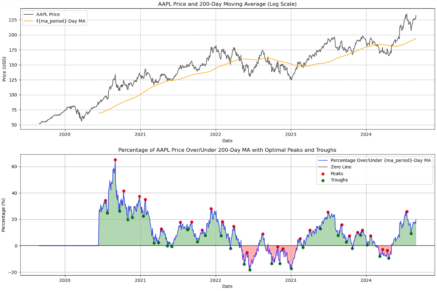
APPLE stock and it’s elasticity indicator — APPLE oscillates between +20% and -20% in most time
The Rubber Band Analogy
Let’s magine a moving average as a rubber band stretched across a chart. The stock price, represented by the current market price, moves above and below this band as in the above chart. Like a rubber band tends to snap back to its resting position when stretched, stock prices often exhibit a tendency to revert to their moving averages over time.
2 Cards Charging 0% Interest Until 2026

Paying down your credit card balance can be tough with the majority of your payment going to interest. Avoid interest charges for up to 18 months with these cards.
Key Components:
Moving Average: Acts as the central point or “resting position” of the rubber band.
Stock Price: Moves dynamically, stretching above or below the moving average.
Elasticity: Varies between different stocks, influencing how far and how quickly prices deviate from and return to the moving average.
Elasticity of Stock
To study the entry and exit of using this rubber band effect, we need to identfiy the pattern when the peak and trough happens — when the price will likely to be snapped back to the moving average from above or below the moving average, as each stock has different ‘elasticity’.
Let’s take a look at a few example of stock of different segments. I further add a subplot to indicate the return of using this strategy … If an investor can “accurately time” the market by buying at troughs (green dots) when the stock rebounds and selling and wait when it peaks (red dots) using this indicator, the potential returns could significantly outperform a traditional buy-and-hold strategy, potentially multiplying the initial investment several times over!!
We cannot simply apply a +10% / -10% or any percentage universally as each stock has different elasticity. We can’t simply define the over sold and over bought level like RSI’s 30/70 rules. We must try to identify the stock’s peak and trough from it’s historical behavior around the moving average.
But how can we identify the peaks and troughs to predict when the price will snap back?
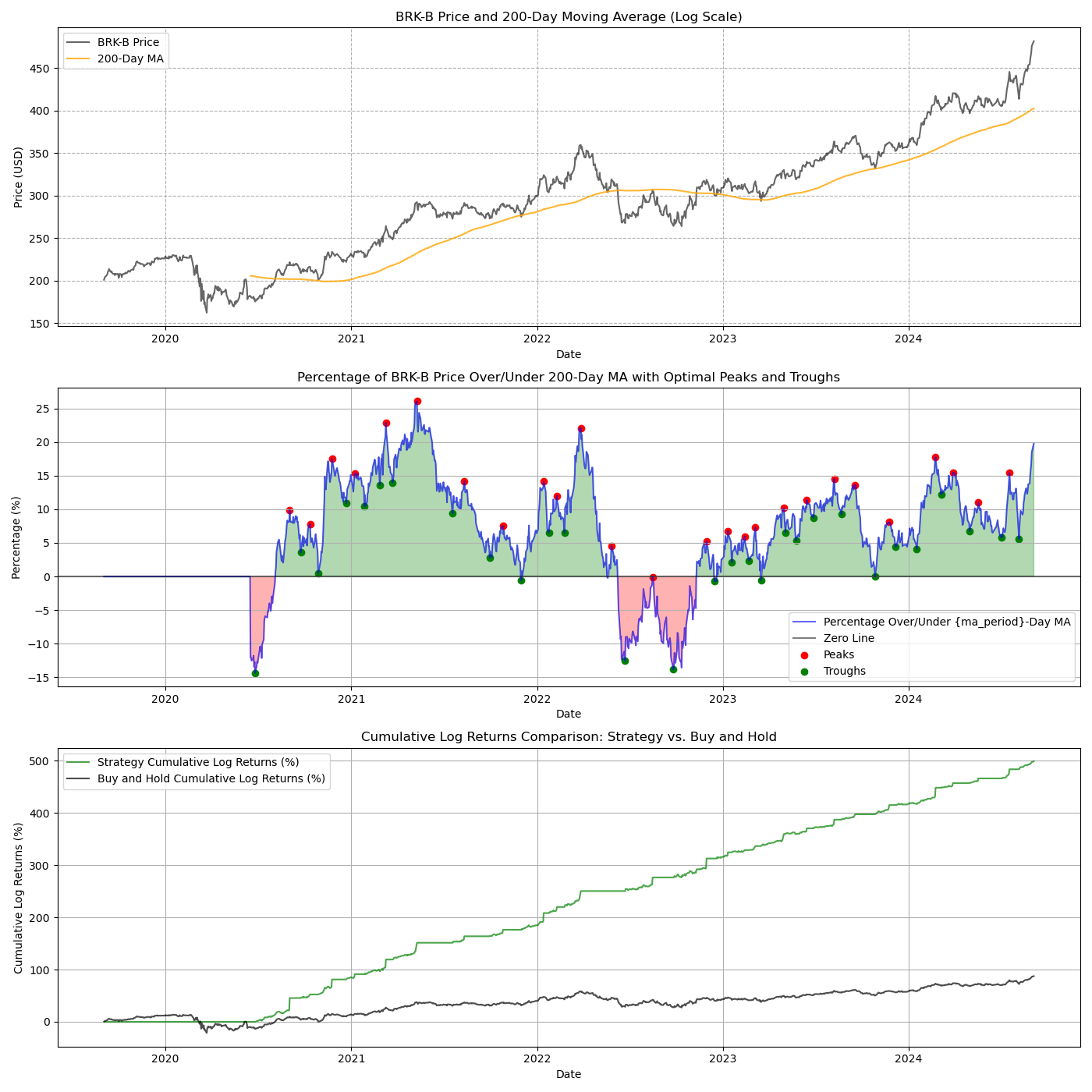
Berkshire Hathaway (class B) has +15% — -15% elasticity
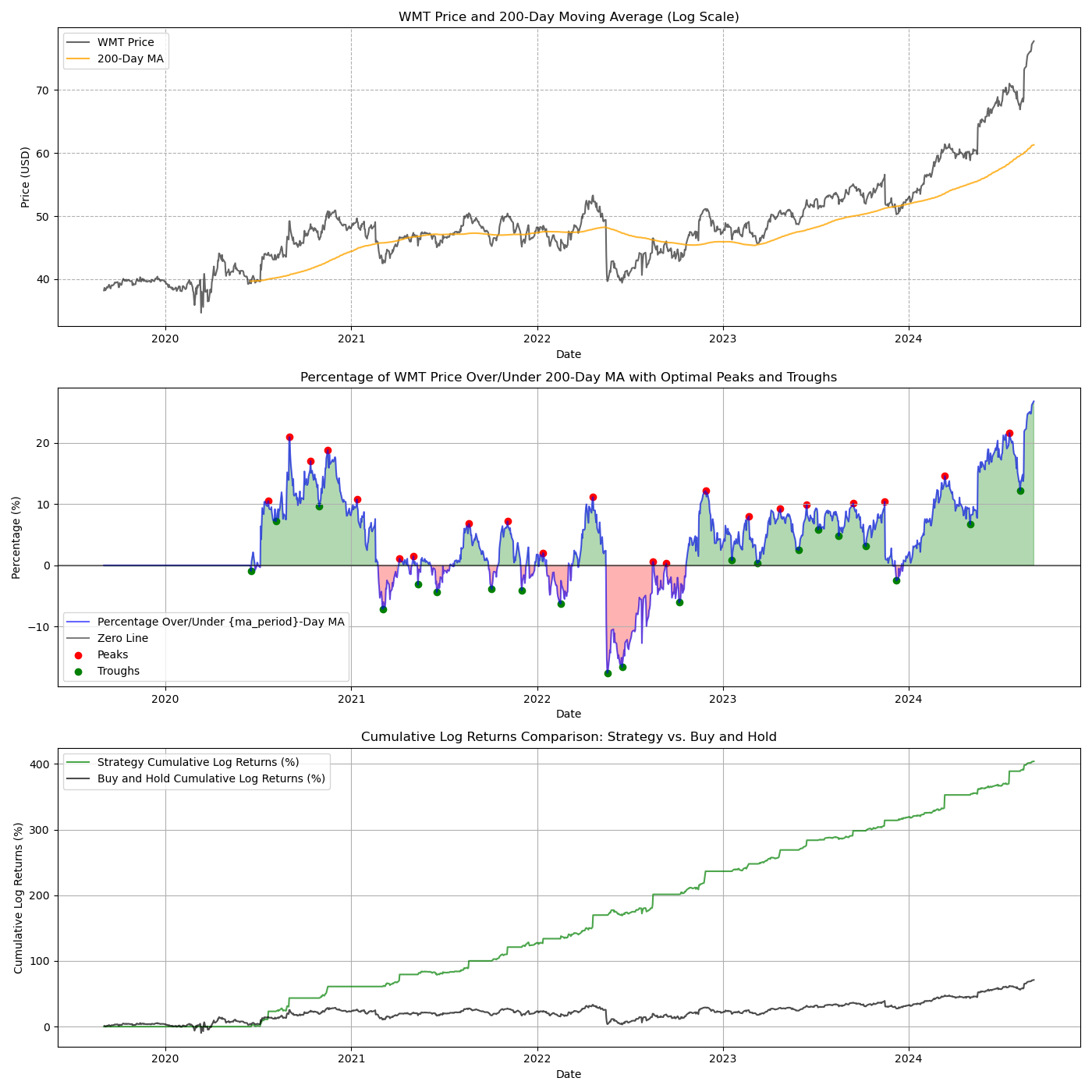
WALMART elasticity is at +10% — -5% in most times
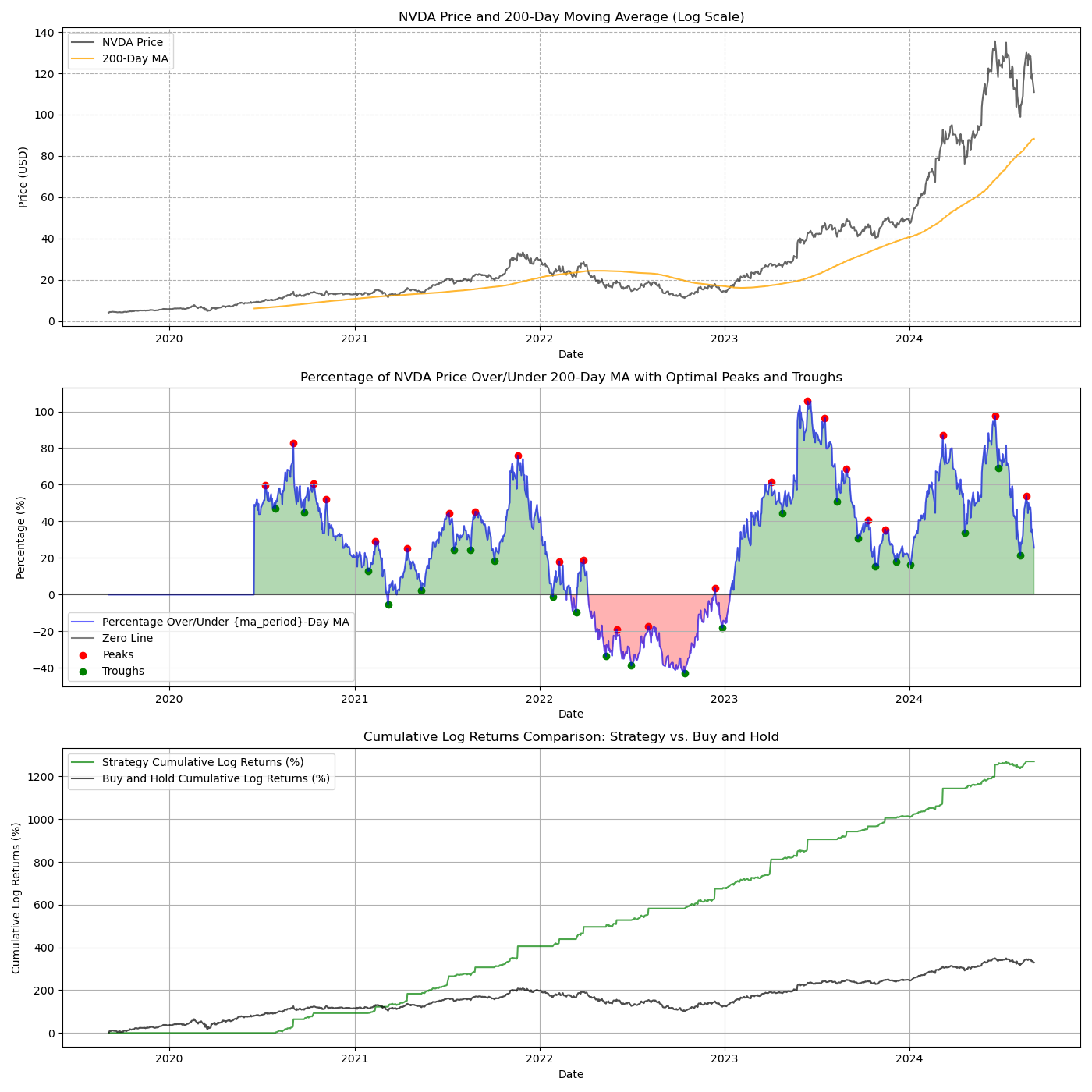
Nvidia has +40% — -40% elasticity and can even goes up to +80–100%!
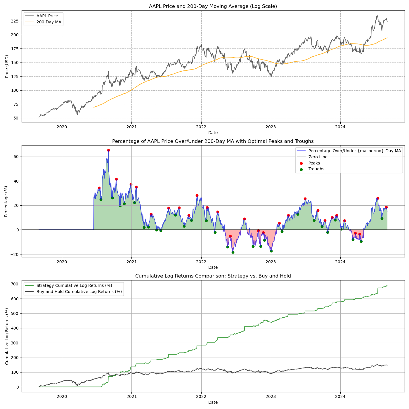
Apple Stock with the potential return if we can follow the Peak and Trough indicator
Photo by Bhautik Patel on Unsplash
Introducing the Neural Network Model
To better explore the rubber band effect and its implications, I try to use a neural network model. The goal of this model is to predict stock price movements in relation to the moving average and identify optimal points of reversion — where the price is likely to revert to the mean or deviate further.
Why Neural Network ?
Stock prices are influenced by numerous factors, making their movements highly non-linear and complex. Neural networks are well-suited to capture these non-linear relationships, making them ideal for predicting price movements that oscillate around moving averages. By training on historical data, the model learns patterns that may indicate the likelihood of price reversion or continuation.
The input to the neural network is not the stock price, but the % of the price above or below the 200 Moving Average. You can test the code by using shorter or longer moving average over a shorter or longer period of course.
Neural Network Architecture:
The Model
The model is a simple feedforward neural network with three layers:
Input Layer: Takes the last 200 days of deviation data as input.
Hidden Layers: Two dense layers with ReLU activation and dropout for regularization. The layers will try to capture complex relationships in the data.
Output Layer: Predicts two key values — window_peak and window_trough, which represent the optimal lookback periods to identify local maxima (peaks) and minima (troughs) in the price data.
Here is the visual representation of the network, I used plot_model to obtain such image:
 from keras.utils import plot_model
 plot_model(model, to_file='model_plot.png', show_shapes=True, show_layer_names=True)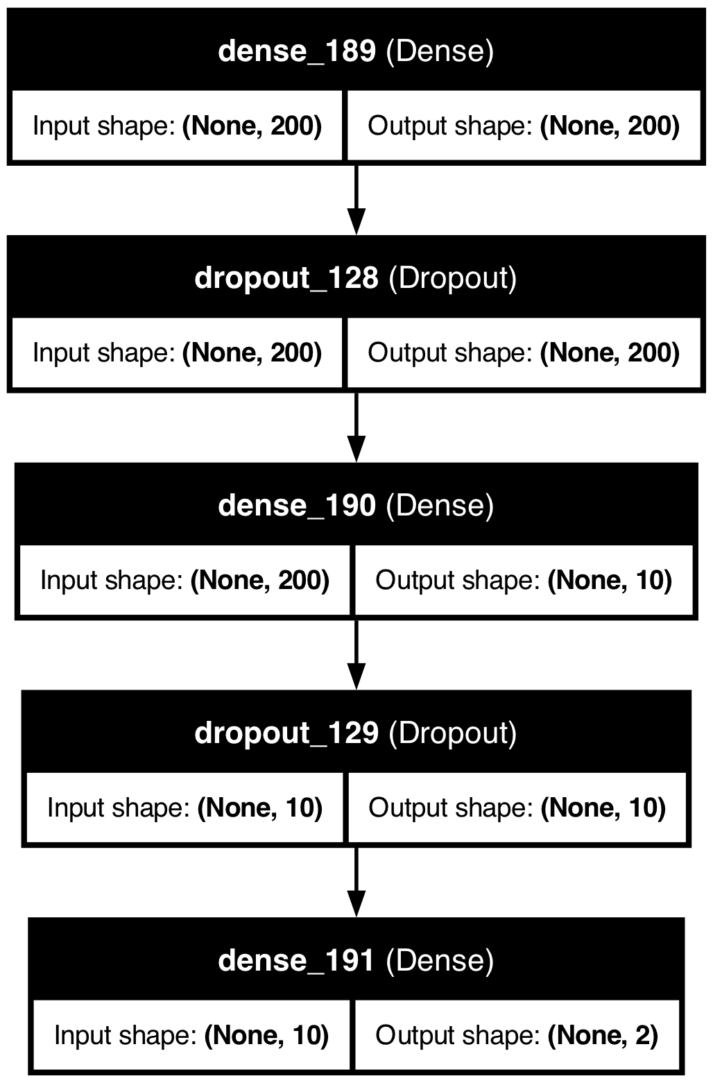
Neural Network architecture for the training
Training
The model is trained using historical data, with random values as the target. The model learns to adjust its predictions to minimize the mean squared error between the predicted peaks/troughs and the actual data.
We split the data into training and testing sets, with the model training on 50% of the data and validating on the remaining.
Prediction and Strategy Implementation:
After training, the model predicts the optimal lookback periods for identifying peaks and troughs in the stock price.
Using these predictions, we identify local maxima and minima in the percentage deviation from the moving average.
A simple trading strategy is then simulated: buy at predicted troughs, sell at predicted peaks, and remain in cash in between.
WARNING: If one decided to enter a trade as soon as a peak or trough signal is identified, we need to wait for confirmation and set cut lost at the signaled peal/trough. It is because even though the peak/trough has appeared, if the following trading day(s) reverse and create a higher peak or lower trough, the signal will be cancelled or readjusted. That’s why using the signal as cut loss will help to minimize lost due to false positive. Split your trade proportionally and control the loss and average in average out is always a better trading strategy.
Conclusion: Insights and Implications
1. Mean Reversion Insights
The model’s predictions offer a dynamic approach to identifying points of reversion in stock prices. Unlike static moving averages, which treat all deviations equally, the model adapts to the data and highlights periods where reversion is more likely, potentially offering more accurate entry and exit points. Please test it out yourself with different timeframe and stock if you would like to verify this. :)
2. Volatility Assessment
Every stock behaves differently, we can’t simply apply Moving Average with xx days, RSI 14 with 30/70 as over sold/over bought signal, etc. We cannot just apply same indicator same parameters and apply to ALL stocks!
By learning the elasticity of price movements around the moving average, the model can help assess the volatility of a stock individually. Stocks with wider oscillations might be more volatile, and the model can adapt its predictions accordingly, offering unique insights per underlying asset.
3. Risk Management
The trading strategy derived from the model’s predictions provides a framework for managing risk. By identifying optimal points to enter and exit trades, the strategy can enhance returns while reducing exposure to adverse price movements.
4. Better than Buy and Hold
The results showed that a strategy based on the model’s predictions could outperform a simple buy-and-hold approach under certain market conditions. However, like all models and other articles I have written, it has limitations and should be used in conjunction with other analysis tools.
Below code should be self explained with comments.
import yfinance as yf
import matplotlib.pyplot as plt
import numpy as np
from scipy.signal import argrelextrema
from keras.models import Sequential
from keras.layers import Dense, Dropout
from sklearn.preprocessing import MinMaxScaler
from keras.utils import plot_model
import sys
from datetime import datetime, date

today = str(date.today())

# Define the stock ticker and the moving average period
ticker = 'AAPL'
ma_period = 200

# Fetch historical data for the last 2 years
stock_data = yf.download(ticker, period="5y")
if len(stock_data) < ma_period:
    sys.exit(f'Data size too small for {ticker}, program aborted.')

# Calculate the xx-day Moving Average (x_day_MA)
stock_data['x_day_MA'] = stock_data['Close'].rolling(window=ma_period).mean()

# Adjust the percentage over/under x-MA calculation
stock_data['Pct_Over_MA'] = (stock_data['Close'] - stock_data['x_day_MA']) / stock_data['x_day_MA'] * 100

# Handle NaN values
stock_data['Pct_Over_MA'].fillna(0, inplace=True)

# Prepare data for neural network
def prepare_data(stock_data, ma_period):
    X = []
    for i in range(ma_period, len(stock_data)):
        X.append(stock_data['Pct_Over_MA'].iloc[i-ma_period:i].values)
    X = np.array(X)

    # Normalize the data
    scaler = MinMaxScaler(feature_range=(0, 1))
    X = scaler.fit_transform(X)

    return X

# Create the neural network model
def build_model(input_dim):
    model = Sequential()
    model.add(Dense(200, input_dim=input_dim, activation='relu', kernel_regularizer='l2'))
    model.add(Dropout(0.3))
    model.add(Dense(10, activation='relu', kernel_regularizer='l2'))
    model.add(Dropout(0.3))
    model.add(Dense(2, activation='linear'))  # Two outputs: window_peak and window_trough
    model.compile(optimizer='adam', loss='mse')
    plot_model(model, to_file='model_plot.png', show_shapes=True, show_layer_names=True)
    return model

# Prepare the data
X = prepare_data(stock_data, ma_period)

# Split the data into training and testing sets
split_index = int(0.5 * len(X))  # 50/50 training vs testing data
X_train, X_test = X[:split_index], X[split_index:]

# Target values (y) are not predefined; the model will attempt to learn the best window_peak and window_trough
y_train = np.random.rand(len(X_train), 2) * 30  # Random values between 0 and 30
y_test = np.random.rand(len(X_test), 2) * 30

# Build and train the model
model = build_model(X_train.shape[1])
history = model.fit(X_train, y_train, epochs=50, batch_size=32, verbose=1, validation_split=0.2)

# Make predictions
predictions = model.predict(X_test)

# Safeguard against NaNs in predictions
def safe_convert_to_int(value):
    if np.isnan(value) or value <= 0:
        return 1  # Default to a safe value
    else:
        return int(value)

best_window_peak = safe_convert_to_int(predictions[-1][0])
best_window_trough = safe_convert_to_int(predictions[-1][1])

# Find local maxima and minima using the predicted optimal windows
local_maxima = argrelextrema(stock_data['Pct_Over_MA'].values, comparator=np.greater, order=best_window_peak)[0]
local_minima = argrelextrema(stock_data['Pct_Over_MA'].values, comparator=np.less, order=best_window_trough)[0]

# Extract peak and trough values
peak_values = stock_data['Pct_Over_MA'].iloc[local_maxima]
trough_values = stock_data['Pct_Over_MA'].iloc[local_minima]

# Initialize positions array
positions = np.zeros(len(stock_data))

# Define buy and sell signals based on local minima and maxima
for i in range(1, len(stock_data)):
    if i in local_minima:
        positions[i] = 1  # Buy
    elif i in local_maxima:
        positions[i] = -1  # Sell

# Calculate log returns for buy and hold
stock_data['Log_Return_BnH'] = np.log(stock_data['Close'] / stock_data['Close'].shift(1))

# Initialize strategy returns with zeros (log returns start at 0)
strategy_log_returns = np.zeros_like(stock_data['Close'].values)

in_position = False
buy_price = 0

for i in range(1, len(stock_data)):
    if positions[i] == 1 and not in_position:
        # Buy at the closing price
        buy_price = stock_data['Close'].iloc[i]
        in_position = True
        strategy_log_returns[i] = strategy_log_returns[i-1]  # Carry forward previous return
    elif positions[i] == -1 and in_position:
        # Sell at the closing price
        sell_price = stock_data['Close'].iloc[i]
        # Calculate the log return for the sell action
        strategy_log_returns[i] = strategy_log_returns[i-1] + np.log(sell_price / buy_price)
        in_position = False
    elif in_position:
        # Update log returns while holding the position
        current_price = stock_data['Close'].iloc[i]
        daily_log_return = np.log(current_price / stock_data['Close'].iloc[i-1])
        strategy_log_returns[i] = strategy_log_returns[i-1] + daily_log_return
    else:
        # Carry forward the previous return if not in position
        strategy_log_returns[i] = strategy_log_returns[i-1]

# Calculate cumulative log returns for buy and hold strategy
stock_data['Cumulative_Log_Return_BnH'] = stock_data['Log_Return_BnH'].cumsum()

# The log returns for the strategy are already cumulative (as we sum them up)
cumulative_strategy_log_returns = strategy_log_returns

# Plot the results
fig = plt.figure(figsize=(14, 7))

# Plot cumulative log returns
plt.plot(stock_data.index, cumulative_strategy_log_returns * 100, label='Strategy Cumulative Log Returns (%)', color='green', alpha=0.7)
plt.plot(stock_data.index, stock_data['Cumulative_Log_Return_BnH'] * 100, label='Buy and Hold Cumulative Log Returns (%)', color='black', alpha=0.7)

plt.title('Cumulative Log Returns Comparison: Strategy vs. Buy and Hold')
plt.xlabel('Date')
plt.ylabel('Cumulative Log Returns (%)')
plt.legend()
plt.grid(True)

# Show the plot
plt.tight_layout()
plt.show()


# Plot the results
fig=plt.figure(figsize=(14, 14))

# First subplot: Stock Price and x-Day MA
ax1 = plt.subplot(3, 1, 1)
plt.plot(stock_data.index, stock_data['Close'], label=f'{ticker} Price', color='black',alpha=0.6)
plt.plot(stock_data.index, stock_data['x_day_MA'], label=f'{ma_period}-Day MA', color='orange', alpha=0.8)
plt.title(f'{ticker} Price and {ma_period}-Day Moving Average (Log Scale)')
plt.xlabel('Date')
plt.ylabel('Price (USD)')
plt.legend()
plt.grid(True, which="both", ls="--")

# Second subplot: Percentage Over/Under x-Day MA with Peaks and Troughs
ax2 = plt.subplot(3, 1, 2, sharex=ax1)
plt.plot(stock_data.index, stock_data['Pct_Over_MA'], label='Percentage Over/Under {ma_period}-Day MA', color='blue', alpha=0.6)
plt.axhline(y=0, color='black', linestyle='-', alpha=0.5, label=f'Zero Line')

# Fill green above 0 and red below 0
plt.fill_between(stock_data.index, stock_data['Pct_Over_MA'], where=(stock_data['Pct_Over_MA'] >= 0), color='green', alpha=0.3)
plt.fill_between(stock_data.index, stock_data['Pct_Over_MA'], where=(stock_data['Pct_Over_MA'] < 0), color='red', alpha=0.3)

plt.scatter(stock_data.index[local_maxima], peak_values, color='red', label='Peaks', marker='o')
plt.scatter(stock_data.index[local_minima], trough_values, color='green', label='Troughs', marker='o')
plt.title(f'Percentage of {ticker} Price Over/Under {ma_period}-Day MA with Optimal Peaks and Troughs')
plt.xlabel('Date')
plt.ylabel('Percentage (%)')
plt.legend()
plt.grid(True)

# Plot cumulative log returns
ax3 = plt.subplot(3, 1, 3, sharex=ax1)

plt.plot(stock_data.index, cumulative_strategy_log_returns * 100, label='Strategy Cumulative Log Returns (%)', color='green', alpha=0.7)
plt.plot(stock_data.index, stock_data['Cumulative_Log_Return_BnH'] * 100, label='Buy and Hold Cumulative Log Returns (%)', color='black', alpha=0.7)

plt.title('Cumulative Log Returns Comparison: Strategy vs. Buy and Hold')
plt.xlabel('Date')
plt.ylabel('Cumulative Log Returns (%)')
plt.legend()
plt.grid(True)

plt.tight_layout()
plt.show()
This Smart Home Company is Growing 200% Month-Over-Month
Ever thought the smartest part of your home could be your window shades?
Meet RYSE, the company transforming ordinary blinds into cutting-edge smart home devices. With 10 granted patents, a major win against copycat sellers on Amazon, and products already featured in 127 Best Buy locations, RYSE is scaling rapidly in a market growing 23% annually.
And they’re just getting started. With 200% month-over-month revenue growth, international expansion on the horizon, and partnerships with retail giants like Home Depot and Lowe’s, RYSE is poised to redefine home automation.
Now, for just $1.75 per share, you can invest in this fast-growing company and be part of the smart home revolution.