Exciting News: Paid Subscriptions Have Launched! 🚀

Last Sunday, we officially rolled out our new paid subscription plans at GuruFinance Insights, offering you the chance to take your investing journey to the next level! For those of you, who already obtained the premium subscription, will start receiving paid content since Tuesday, September 3. Whether you're just starting or are a seasoned trader, these plans are packed with exclusive trading strategies, in-depth research paper analysis, ad-free content, monthly AMA sessions, coding tutorials for automating trading strategies, and much more.

Our three tailored plans—Starter Investor, Pro Trader, and Elite Investor—provide a range of valuable tools and personalized support to suit different needs and goals. Don’t miss this opportunity to get real-time trade alerts, access to masterclasses, one-on-one strategy consultations, and be part of our private community group. Click here to explore the plans and see how becoming a premium member can elevate your investment strategy!

🗣️ Stock Market Today: Blackstone to buy Australia's AirTrunk in $16 billion deal

Blackstone, in partnership with the Canada Pension Plan Investment Board (CPP Investments), will acquire Australian data center group AirTrunk for an enterprise value exceeding A$24 billion ($16.1 billion), marking Blackstone's largest investment in the Asia Pacific region. The deal, which is the largest buyout in Australia this year, requires approval from the Australian Foreign Investment Review Board due to the involvement of overseas buyers. AirTrunk, founded in Sydney in 2015, is the largest data center group in Asia Pacific, with 11 sites across Australia, Japan, Malaysia, Hong Kong, and Singapore. The acquisition sees AirTrunk's previous majority owners, Macquarie Asset Management and Canada's Public Sector Pension Investment Board, selling their entire stake, while founder and CEO Robin Khuda will retain a portion of his shareholding and continue leading the company.

The value of AirTrunk increased during the sales process, driven by the growing demand for digital infrastructure fueled by the artificial intelligence (AI) boom. CPP Investments, which will hold a 12% stake in AirTrunk after the transaction is finalized, highlighted the significant growth in the Asia Pacific data center sector, particularly due to AI adoption. Blackstone aims to solidify its position as a leading digital infrastructure investor globally, and this acquisition represents a strategic move in that direction. The Blackstone and CPP Investments group won the bid for AirTrunk, outcompeting a consortium led by IFM Investors.

Stay informed with today's rundown:

Today, we delve into the “Time Series Analysis of Netflix Stocks with Pandas”👇

Time series analysis of data is not just a collection of numbers, in this case Netflix stocks. It is a captivating tapestry that weaves together the intricate story of our world with Pandas. Like a mystical thread, it captures the ebb and flow of events, the rise and fall of trends, and the emergence of patterns. It reveals the hidden connections and correlations that shape our reality, painting a vivid picture of the past and offering glimpses into the future.

Time series analysis is more than just a tool. It is a gateway to a realm of knowledge and foresight. You will be empowered to unlock the secrets hidden within the temporal fabric of data, transforming raw information into valuable insights. Also, guides you in making informed decisions, mitigating risks, and capitalizing on emerging opportunities

Let’s embark on this exciting adventure together and discover how time truly holds the key to understanding our world. Are you ready? Let’s dive into the captivating realm of time series analysis!

Learning Objectives

• We aim to introduce the concept of time series analysis and highlight its significance in various fields and presenting real-world examples that showcase the practical applications of time series analysis.

• We will provide a practical demonstration by showcasing how to import Netflix stock data using Python and yfinance library. So that the readers will learn the necessary steps to acquire time series data and prepare it for analysis.

• Finally, we will focus on important pandas functions used in time series analysis, such as shifting, rolling, and resampling which enables to manipulate and analyze time series data effectively.

What is Time Series Analysis?

A time series is a sequence of data points collected or recorded over successive and equally spaced intervals of time.

• Time series analysis is a statistical technique for analyzing data points collected over time.

• It involves studying patterns, trends, and dependencies in sequential data to extract insights and make predictions.

• It involves techniques such as data visualization, statistical modeling, and forecasting methods to analyze and interpret time series data effectively.

Examples of Time Series Data

1. Stock Market Data: Analyzing historical stock prices to identify trends and forecast future prices.

2. Weather Data: Studying temperature, precipitation, and other variables over time to understand climate patterns.

3. Economic Indicators: Analyzing GDP, inflation rates, and unemployment rates to assess economic performance.

4. Sales Data: Examining sales figures over time to identify patterns and forecast future sales.

5. Website Traffic: Analyzing web traffic metrics to understand user behavior and optimize website performance.

Components of Time Series

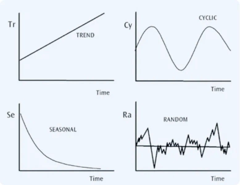
There are 4 Components of Time Series. They are:

• Trend Component: The trend represents a long-term pattern in the data that moves in a relatively predictable manner either upward or downward.

• Seasonality Component: The seasonality is a regular and periodic pattern that repeats itself over a specific period, such as daily, weekly, monthly, or seasonally.

• Cyclical Component: The cyclical component corresponds to patterns that follow business or economic cycles, characterized by alternating periods of growth and decline.

• Random Component: The random component represents unpredictable and residual fluctuations in the data that do not conform to the trend, seasonality, or cyclical patterns.

Here is a visual interpretation of the various components of the Time Series.

Working with yfinance in Python

Let’s now see a practical use of yfinance. First, we will download the yfinance library using the following command.

Installation

!pip install yfinance

Please be aware that if you encounter any errors while running this code on your local machine, such as in Jupyter Notebook, you have two options: either update your Python environment or consider utilizing cloud-based notebooks like Google Colab. as an alternative solution.

Import Libraries

import pandas as pd
import matplotlib.pyplot as plt
import yfinance as yf
from datetime import datetime

Download Netflix Financial Dataset Using Yahoo Finance

In this demo, we will be using the Netflix’s Stock data(NFLX)

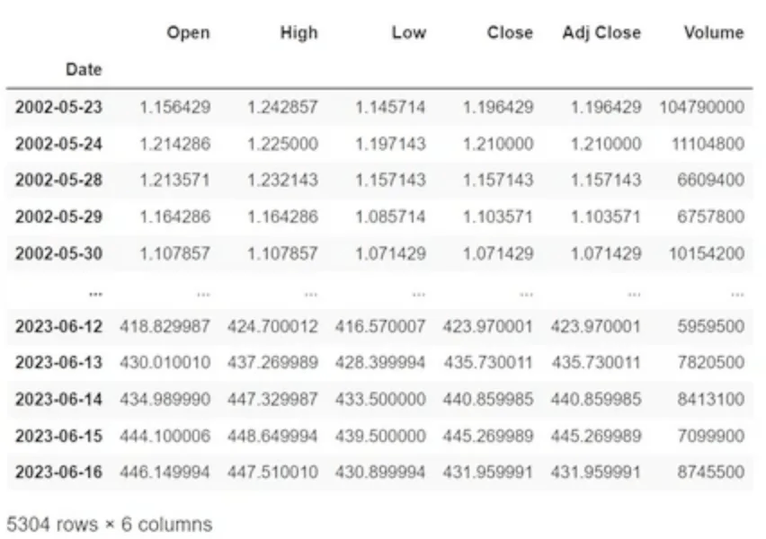
df =  yf.download(tickers = "NFLX")
df

Let’s examine the columns in detail for further analysis:

• The “Open” and “Close” columns show the opening and closing prices of the stocks on a specific day.

• The “High” and “Low” columns indicate the highest and lowest prices reached by the stock on a particular day, respectively.

• The “Volume” column provides information about the total volume of stocks traded on a specific day.

• The “Adj_Close” column represents the adjusted closing price, which reflects the stock’s closing price on any given trading day, considering factors such as dividends, stock splits, or other corporate actions.

About the Data

# print the metadata of the dataset
df.info()

# data description
df.describe()

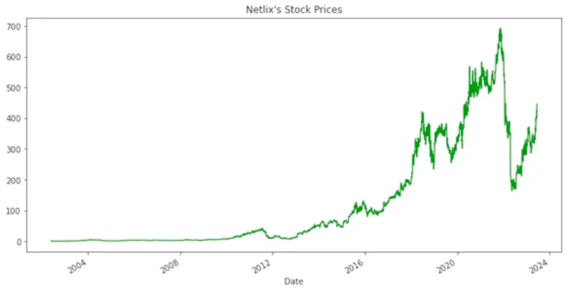
Visualizing the Time Series data

df['Open'].plot(figsize=(12,6),c='g')
plt.title("Netlix's Stock Prices")
plt.show()

There has been a steady increase in Netflix’s Stock Prices from 2002 to 2021.We shall use Pandas to investigate it further in the coming sections.

Pandas for Time Series Analysis

Due to its roots in financial modeling, Pandas provides a rich array of tools for handling dates, times, and time-indexed data. Now, let’s explore the key Pandas data structures designed specifically for effective manipulation of time series data.

1. Time Shifting

Time shifting, also known as lagging or shifting in time series analysis, refers to the process of moving the values of a time series forward or backward in time. It involves shifting the entire series by a specific number of periods.

Presented below is the unaltered dataset prior to any temporal adjustments or shifts:

There are two common types of time shifting:

1.1 Forward Shifting(Positive Lag)

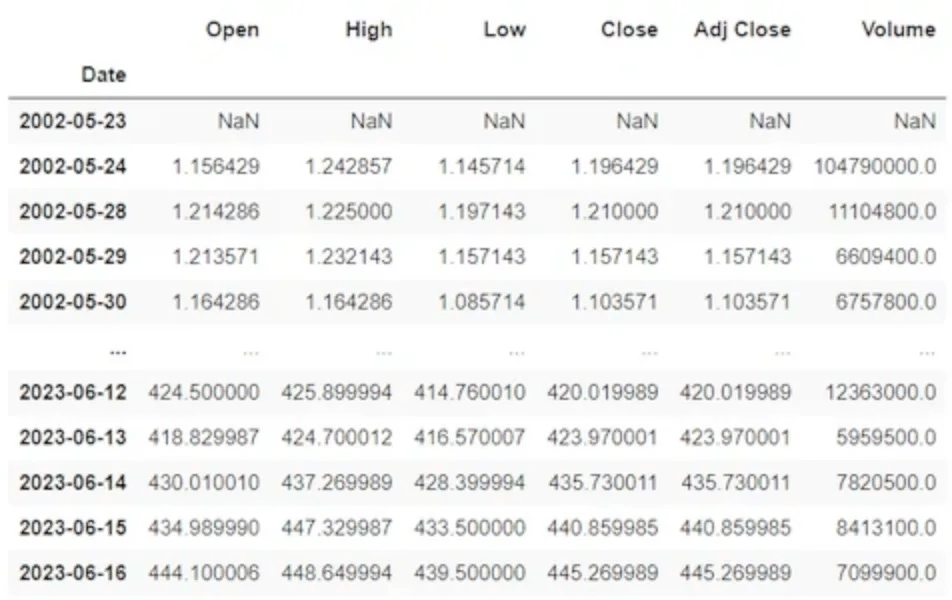
To shift our data forwards, the number of periods (or increments) must be positive.

df.shift(1)

Note: The first row in the shifted data contains a NaN value since there is no previous value to shift it from.

1.2 Backward Shifting(Negative Lag)

To shift our data backwards, the number of periods (or increments) must be negative.

df.shift(-1)

Note: The last row in the shifted data contains a NaN value since there is no subsequent value to shift it from.

2. Rolling Windows

Rolling is a powerful transformation method used to smooth out data and reduce noise. It operates by dividing the data into windows and applying an aggregation function, such as

mean(), median(), sum(), etc. to the values within each window.

df['Open:10 days rolling'] = df['Open'].rolling(10).mean()
df[['Open','Open:10 days rolling']].head(20)
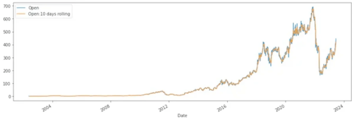
df[['Open','Open:10 days rolling']].plot(figsize=(15,5))
plt.show()

Note: The first nine values have all become blank as there wasn’t enough data to actually fill them when using a window of ten days.

df['Open:20'] = df['Open'].rolling(window=20,min_periods=1).mean()
df['Open:50'] = df['Open'].rolling(window=50,min_periods=1).mean()
df['Open:100'] = df['Open'].rolling(window=100,min_periods=1).mean()
#visualization
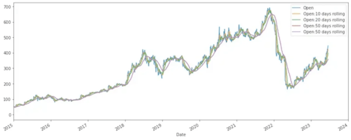
df[['Open','Open:10','Open:20','Open:50','Open:100']].plot(xlim=['2015-01-01','2024-01-01'])
plt.show()

They are commonly used to smoothen plots in time series analysis. The inherent noise and short-term fluctuations in the data can be reduced, allowing for a clearer visualization of underlying trends and patterns.

3. Time Resampling

Time resampling involves aggregating data into predetermined time intervals, such as monthly, quarterly, or yearly, to provide a summarized view of the underlying trends. Instead of examining data on a daily basis, resampling condenses the information into larger time units, allowing analysts to focus on broader patterns and trends rather than getting caught up in daily fluctuations.

#year end frequency
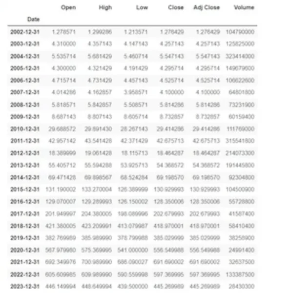
df.resample(rule='A').max()

This resamples the original DataFrame df based on the year-end frequency, and then calculates the maximum value for each year. This can be useful in analyzing the yearly highest stock price or identifying peak values in other time series data.

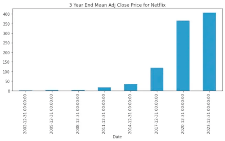
df['Adj Close'].resample(rule='3Y').mean().plot(kind='bar',figsize=(10,4))
plt.title('3 Year End Mean Adj Close Price for Netflix')
plt.show()

This bar plot show the average Adj_Close value of Netflix Stock Price for every 3 years from 2002 to 2023.