
In partnership with

Where Accomplished Wealth Builders Connect, Learn & Grow

Long Angle is a private, vetted community for high-net-worth entrepreneurs and executives. No fees, no pitches—just real peers navigating wealth at your level. Inside, you’ll find:
Self-made professionals, 30–55, $5M–$100M net worth
Confidential conversations, peer advisory groups, live meetups
Institutional-grade investments, $100M+ deployed annually
🚀 Your Investing Journey Just Got Better: Premium Subscriptions Are Here! 🚀
It’s been 4 months since we launched our premium subscription plans at GuruFinance Insights, and the results have been phenomenal! Now, we’re making it even better for you to take your investing game to the next level. Whether you’re just starting out or you’re a seasoned trader, our updated plans are designed to give you the tools, insights, and support you need to succeed.
Here’s what you’ll get as a premium member:
Exclusive Trading Strategies: Unlock proven methods to maximize your returns.
In-Depth Research Analysis: Stay ahead with insights from the latest market trends.
Ad-Free Experience: Focus on what matters most—your investments.
Monthly AMA Sessions: Get your questions answered by top industry experts.
Coding Tutorials: Learn how to automate your trading strategies like a pro.
Masterclasses & One-on-One Consultations: Elevate your skills with personalized guidance.
Our three tailored plans—Starter Investor, Pro Trader, and Elite Investor—are designed to fit your unique needs and goals. Whether you’re looking for foundational tools or advanced strategies, we’ve got you covered.
Don’t wait any longer to transform your investment strategy. The last 4 months have shown just how powerful these tools can be—now it’s your turn to experience the difference.
Tesla Double Moving Average Crossover Strategy Chart
Introduction
The Double Moving Average Crossover is one of the simplest yet powerful trading strategies used by both beginners and seasoned traders. By using two different moving averages, this strategy identifies potential buy and sell signals when the faster moving average crosses over or under a slower one. In this article, we’ll dive into the details of how to implement this strategy in Python, backtest it, and analyze the results.
📈 Algorithmic Trading Course — Join the Waitlist
I’m launching a premium online course on algorithmic trading starting July 14. The price is $3000, and spots will be limited.
🔥 What to Expect:
Build trading bots with Python
Backtest strategies with real data
Learn trend-following, mean-reversion, and more
Live execution, portfolio risk management
Bonus: machine learning & crypto trading modules
🎁 Free Bonus:
Everyone who enrolls will get a free e-book:
“100 Trading Strategies in Python” — full of ready-to-use code.
What is a Double Moving Average Crossover?
The Double Moving Average Crossover strategy relies on two exponential moving averages (EMAs):
Short-term Moving Average (fast): This moving average responds quickly to recent price changes.
Long-term Moving Average (slow): This one reacts more slowly to price changes, capturing long-term trends.
Key Signals:
Buy Signal: When the short-term EMA crosses above the long-term EMA, indicating an upward trend.
Sell Signal: When the short-term EMA crosses below the long-term EMA, indicating a downward trend.
This strategy works well in trending markets but may generate false signals during sideways (range-bound) markets.
Advantages
Simplicity: The strategy’s logic is straightforward and easy to understand, making it accessible for traders with varying levels of experience.
Trend-Following: By identifying crossovers, the strategy aligns with prevailing trends, making it effective in trending markets where it can capture substantial price movements.
Reduced Emotional Bias: Using systematic moving average rules helps traders reduce emotional bias, leading to more consistent decision-making.
Customizable: Moving averages can be adjusted based on time frames and trading goals, allowing for flexibility across different asset classes and market conditions.
Disadvantages
Lagging Indicators: Moving averages are inherently lagging, so this strategy often signals a buy or sell after the trend has begun. This lag can result in delayed entry or exit.
False Signals in Range-Bound Markets: In sideways or range-bound markets, the crossover signals can be frequent and misleading, leading to “whipsaw” trades and potential losses.
Limited Predictive Power: Since moving averages are calculated based on historical prices, they do not predict future prices but rather follow the trend, which may be unsuitable for highly volatile markets.
Important Considerations
Time Frame Selection: The moving average lengths you choose greatly affect the strategy’s performance. Shorter moving averages provide more frequent signals but increase the chance of false signals, while longer moving averages are more stable but may miss shorter trends.
Market Conditions: This strategy is most effective in trending markets. In range-bound conditions, additional filters (like using volume or other indicators) may help to avoid false signals.
Risk Management: As with any trading strategy, risk management techniques like setting stop losses and using position sizing are essential to protect capital.
Backtesting and Optimization: Regularly backtesting and fine-tuning this strategy with historical data helps to understand how it performs under different market conditions, making it more reliable for real-world trading.
Simulate the Strategy in Python
We now simulate the Double Moving Average Crossover Strategy on historical data.
Setting Up the Environment
To implement this strategy, you’ll need Python along with a few essential libraries. In your python environment, install the following libraries:
pip install pandas numpy matplotlib yfinanceImporting Libraries
Import the libraries in a .ipynb notebook:
import pandas as pd
import numpy as np
import matplotlib.pyplot as plt
import yfinance as yf
from tabulate import tabulate
from datetime import datetime
Data
We’ll use historical data from Yahoo Finance to apply our strategy. For this example, let’s use Tesla’s stock (TSLA).
# Define the stock symbol and the date range for our data
stock_symbol = 'TSLA'
start_date = '2024-01-01'
end_date = datetime.today().strftime('%Y-%m-%d')  # Sets end date to today's date
print(f"Double Moving Average Crossover Trading for: {stock_symbol}\nStart Date: {start_date}\nEnd Date: {end_date}")
After downloading the data, we can now preprocess it for easy strategy simulation:
df = yf.download(stock_symbol, start=start_date, end=end_date)

# Select the desired columns (first level of MultiIndex)
df.columns = df.columns.get_level_values(0)

# Keep only the columns you are interested in
df = df[['Open', 'Close', 'Volume', 'Low', 'High']]

# If the index already contains the dates, rename the index
df.index.name = 'Date'  # Ensure the index is named "Date"

# Resetting the index if necessary
df.reset_index(inplace=True)

# Ensure that the index is of type datetime
df['Date'] = pd.to_datetime(df['Date'])

# Set the 'Date' column as the index again (in case it's reset)
df.set_index('Date', inplace=True)

df.head()
Visualize the Chart
# Plot the closing price
plt.figure(figsize=(12, 6))

plt.plot(df['Close'], label='Closing Price')

# Add title, labels, and legend
plt.title(f'{stock_symbol} Closing Price')
plt.xlabel('Date')
plt.ylabel('Price ($)')
plt.legend()

# Save the plot in 300dpi
plt.savefig(f'{stock_symbol}_stock_chart.png', dpi=300)

# Show the plot
plt.show()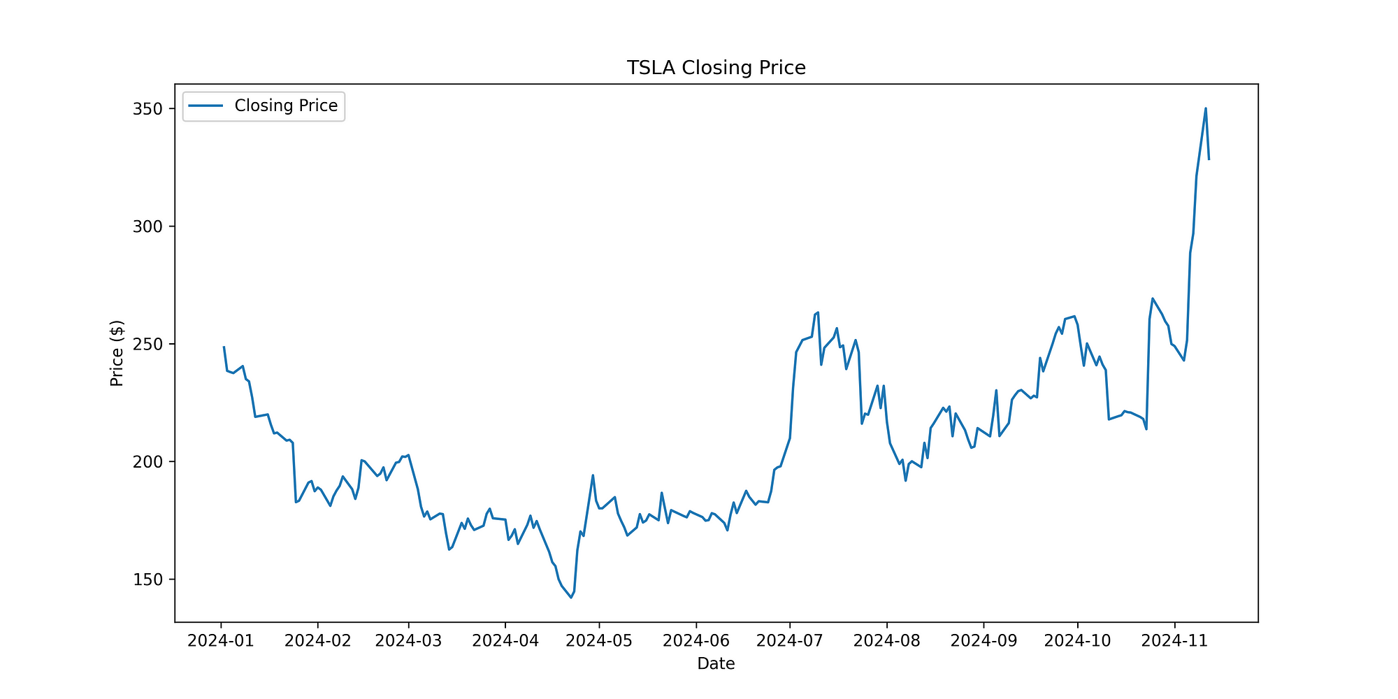
Tesla Stock Price Chart
Calculating Moving Averages
In this section, we calculate the short-term and long-term Exponential Moving Averages (EMAs) using two window sizes, a long and short window. The short-term EMA reacts faster to recent price changes, while the long-term EMA smooths out fluctuations to highlight longer-term trends. These moving averages help in identifying crossover points for potential buy and sell signals.
# Calculate the short and long EMAs
SHORT_WINDOW = 10
LONG_WINDOW = 30
df['SHORT_WINDOW'] = df['Close'].ewm(span=SHORT_WINDOW, adjust=False).mean()
df['LONG_WINDOW'] = df['Close'].ewm(span=LONG_WINDOW, adjust=False).mean()
Visualize the Moving Averages
# Plot the Close Price and EMAs
plt.figure(figsize=(14, 7))

# Plot Close Price
plt.plot(df.index, df['Close'], label='Close Price', linewidth=2)

# Plot Short-term EMA
plt.plot(df.index, df['SHORT_WINDOW'], label=f'{SHORT_WINDOW}-day EMA', linestyle='--')

# Plot Long-term EMA
plt.plot(df.index, df['LONG_WINDOW'], label=f'{LONG_WINDOW}-day EMA', linestyle='--')

# Labels and title
plt.xlabel('Date')
plt.ylabel('Price ($)')
plt.title(f'{stock_symbol} Close Price with Short and Long EMAs')
plt.legend()

# Save plot in 300dpi
plt.savefig(f'{stock_symbol}_moving_averages.png', dpi=300)

plt.show()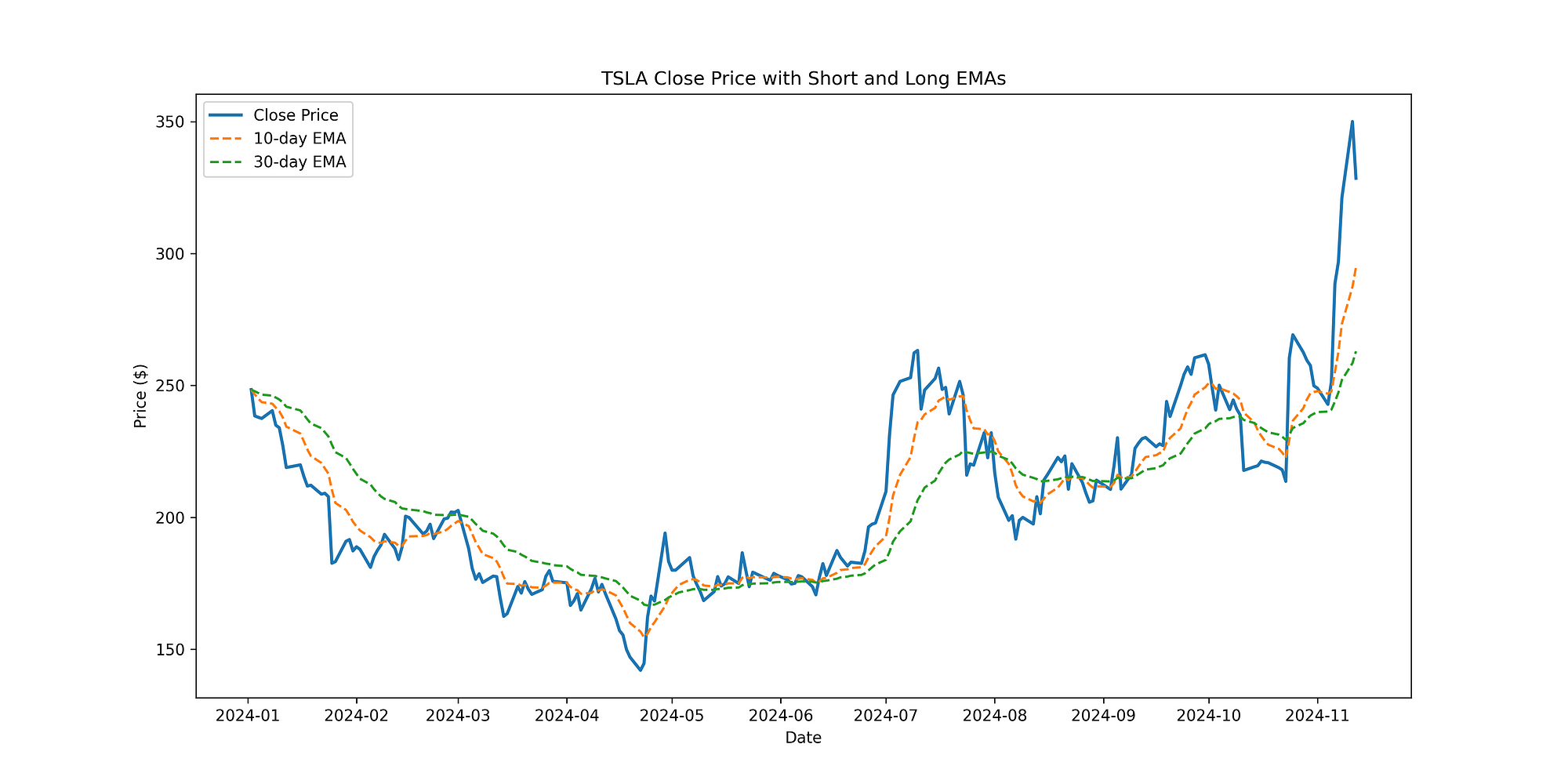
Tesla Stock Chart with Moving Averages
Creating Buy and Sell Signals
We’ll add a Signal column to store buy and sell signals based on crossover points.
# Generate buy and sell signals in a single column
df['Signal'] = np.where(
    (df['SHORT_WINDOW'] > df['LONG_WINDOW']) & (df['SHORT_WINDOW'].shift(1) <= df['LONG_WINDOW'].shift(1)), 1,  # Buy Signal
    np.where(
        (df['SHORT_WINDOW'] < df['LONG_WINDOW']) & (df['SHORT_WINDOW'].shift(1) >= df['LONG_WINDOW'].shift(1)), -1,  # Sell Signal
        0  # No Signal
    )
)
Simulate the Strategy
Calculate the Brokerage Fee
We define a function to calculate the brokerage fee for each transaction. The fee is set to 0.25% of the transaction amount, with a minimum fee of $0.01 to ensure that small transactions still incur a reasonable fee. This helps simulate the costs associated with trading, making the strategy more realistic.
# Define the fee calculation function
def calculate_fee(amount: float) -> float:
    """Calculate the brokerage fee based on transaction amount."""
    fee = amount * 0.0025  # 0.25% of the transaction
    return max(fee, 0.01)   # Minimum fee of $0.01
Run Backtest
# Starting capital
initial_cash = 100  # Example initial capital
cash = initial_cash
shares = 0
df['Portfolio Value'] = cash

# List to store transaction details for tabulation
transaction_details = []

for i, row in df.iterrows():
    if row['Signal'] == 1 and cash > 0:  # Buy condition
        # Calculate the fee for the buy transaction
        fee = calculate_fee(cash)

        # Calculate how many shares can be bought after deducting the fee
        shares_bought = (cash - fee) / row['Close']

        # Deduct the cash and fee for the purchase
        cash -= shares_bought * row['Close'] + fee

        # Add the bought shares to the portfolio
        shares += shares_bought

        # Record transaction details
        transaction_details.append([row.name, 'Buy', round(row['Close'], 2), round(fee, 2), round(cash + (shares * row['Close']), 2)])

    elif row['Signal'] == -1 and shares > 0:  # Sell condition
        # Calculate how much cash is earned from selling shares
        total_sale_amount = shares * row['Close']

        # Calculate the fee for the sell transaction
        fee = calculate_fee(total_sale_amount)

        # Cash earned after the fee is deducted
        cash_earned = total_sale_amount - fee

        # Update the cash balance after selling shares
        cash += cash_earned

        # All shares are sold
        shares = 0

        # Record transaction details
        transaction_details.append([row.name, 'Sell', round(row['Close'], 2), round(fee, 2), round(cash, 2)])

    # Update portfolio value
    df.at[i, 'Portfolio Value'] = cash + (shares * row['Close'])

# Summarize results using tabulate
print(tabulate(transaction_details, headers=["Date", "Action", "Price ($)", "Fee ($)", "Portfolio Value ($)"], tablefmt="pretty"))

# Final performance
final_value = cash + (shares * df.iloc[-1]['Close'])
profit = final_value - initial_cash
print(f"\nFinal Portfolio Value: ${final_value:.2f}")
print(f"Total Profit/Loss: ${profit:.2f}")
Analyzing the Results
Tabulate Buys and Sells
The code above shows a table similar to the one below where they buys and sells are shown alongside their fees and the portfolio value. We can see that this strategy with a SHORT_WINDOW = 10 and LONG_WINDOW = 30 leads to a profit of $21.67 from 01 January 2024 to 13 November 2024 .
+---------------------------+--------+-----------+---------+---------------------+
|           Date            | Action | Price ($) | Fee ($) | Portfolio Value ($) |
+---------------------------+--------+-----------+---------+---------------------+
| 2024-05-01 00:00:00+00:00 |  Buy   |  179.99   |  0.25   |        99.75        |
| 2024-06-11 00:00:00+00:00 |  Sell  |  170.66   |  0.24   |        94.34        |
| 2024-06-12 00:00:00+00:00 |  Buy   |  177.29   |  0.24   |        94.11        |
| 2024-08-05 00:00:00+00:00 |  Sell  |  198.88   |  0.26   |        105.3        |
| 2024-09-05 00:00:00+00:00 |  Buy   |  230.17   |  0.26   |       105.04        |
| 2024-10-15 00:00:00+00:00 |  Sell  |  219.57   |  0.25   |        99.95        |
| 2024-10-25 00:00:00+00:00 |  Buy   |  269.19   |  0.25   |        99.7         |
+---------------------------+--------+-----------+---------+---------------------+

Initial Portfolio Vaue: $100.00
Final Portfolio Value: $121.67
Total Profit/Loss: $21.67
Visualize the Buys and Sells
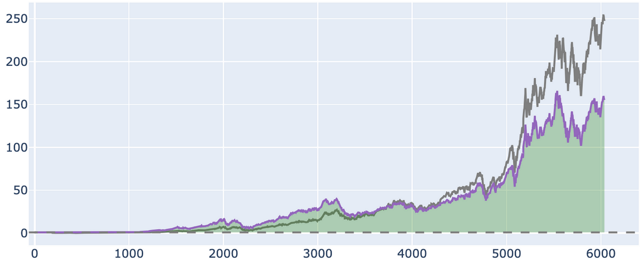
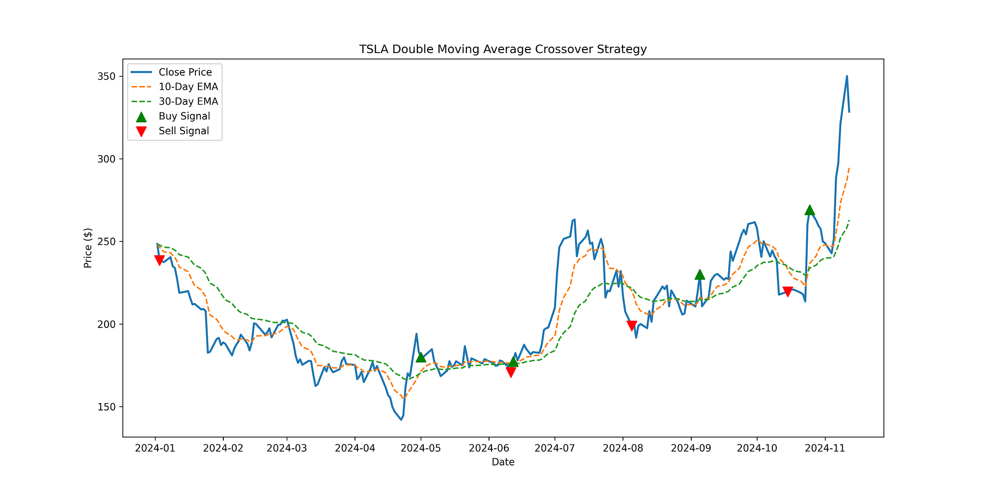
We can now visualize when the buys and sells are made. From this we can adjust our window sizes accordingly.
Tesla Stock Price, Moving Averages and Buy/Sell Signals
Conclusion
The Double Moving Average Crossover Strategy is a straightforward yet effective approach to trading in trending markets. However, remember that no strategy is foolproof. Backtesting on various stocks and timeframes can help you understand how it performs under different market conditions. Implementing a trailing stop or combining this strategy with other indicators like the RSI can further improve its robustness.