
In partnership with

Introducing the first AI-native CRM

Connect your email, and you’ll instantly get a CRM with enriched customer insights and a platform that grows with your business.
With AI at the core, Attio lets you:
Prospect and route leads with research agents
Get real-time insights during customer calls
Build powerful automations for your complex workflows
Join industry leaders like Granola, Taskrabbit, Flatfile and more.
🚀 Your Investing Journey Just Got Better: Premium Subscriptions Are Here! 🚀
It’s been 4 months since we launched our premium subscription plans at GuruFinance Insights, and the results have been phenomenal! Now, we’re making it even better for you to take your investing game to the next level. Whether you’re just starting out or you’re a seasoned trader, our updated plans are designed to give you the tools, insights, and support you need to succeed.
Here’s what you’ll get as a premium member:
Exclusive Trading Strategies: Unlock proven methods to maximize your returns.
In-Depth Research Analysis: Stay ahead with insights from the latest market trends.
Ad-Free Experience: Focus on what matters most—your investments.
Monthly AMA Sessions: Get your questions answered by top industry experts.
Coding Tutorials: Learn how to automate your trading strategies like a pro.
Masterclasses & One-on-One Consultations: Elevate your skills with personalized guidance.
Our three tailored plans—Starter Investor, Pro Trader, and Elite Investor—are designed to fit your unique needs and goals. Whether you’re looking for foundational tools or advanced strategies, we’ve got you covered.
Don’t wait any longer to transform your investment strategy. The last 4 months have shown just how powerful these tools can be—now it’s your turn to experience the difference.
Quantitative finance often begins with randomness but ends with structure. That structure takes the form of partial differential equations (PDEs). These equations describe how the probability of future prices evolves. From stochastic processes, we arrive at PDEs. From PDEs, we find solutions that support option pricing, hedging, and risk management.
Taylor Series and the Idea of Local Approximation
Start with a function f(x). To understand its behavior near a point x_0, we can write:

This local approximation allows us to analyze nonlinear behavior by focusing on the first few derivatives. In finance, we apply this idea to value functions, payoff profiles, and density functions. The second-order term becomes essential when modeling variance, which reflects uncertainty.
Where to Invest $100,000 According to Experts

Investors face a dilemma. Headlines everywhere say tariffs and AI hype are distorting public markets.
Now, the S&P is trading at over 30x earnings—a level historically linked to crashes.
And the Fed is lowering rates, potentially adding fuel to the fire.
Bloomberg asked where experts would personally invest $100,000 for their September edition. One surprising answer? Art.
It’s what billionaires like Bezos, Gates, and the Rockefellers have used to diversify for decades.
Why?
Contemporary art prices have appreciated 11.2% annually on average
…And with one of the lowest correlations to stocks of any major asset class (Masterworks data, 1995-2024).
Ultra-high net worth collectors (>$50M) allocated 25% of their portfolios to art on average. (UBS, 2024)
Thanks to the world’s premiere art investing platform, now anyone can access works by legends like Banksy, Basquiat, and Picasso—without needing millions. Want in? Shares in new offerings can sell quickly but…
*Past performance is not indicative of future returns. Important Reg A disclosures: masterworks.com/cd.

A Taylor Expansion: The second-order expansion shows how we approximate nonlinear functions locally, which underpins the derivation of PDEs in finance.
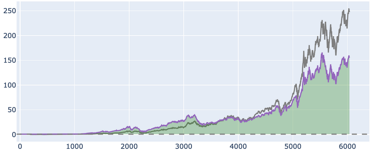
A Trinomial Random Walk
Before jumping into calculus, return to a discrete model. A simple way to represent price evolution is a trinomial tree. At each time step, the price moves up, down, or stays the same:
Up: S→S⋅u
Down: S→S⋅d
No change: S→S
We assign probabilities p_u, p_d, and p_m. The sum equals 1. This random walk converges to a diffusion process as the step size shrinks. The convergence provides the intuition behind stochastic differential equations.
The key is to track the evolution of probability distributions. That leads us to transition density functions.

Trinomial Random Walk: This simulates discrete price evolution, a precursor to continuous stochastic processes.
Transition Density Functions
Let X(t) be a stochastic process. The transition density p(x,t∣x0,t0) gives the probability density of X(t)=x given that X(t0)=x0. For a Markov process, this density contains all the information needed to understand future states.
The transition density evolves over time. Its dynamics can be expressed using a partial differential equation. That equation comes from the underlying stochastic process.
Our First Stochastic Differential Equation
Consider a basic stochastic differential equation (SDE):

Here, μ is the drift, σ is the diffusion, and W_t is a Wiener process. This equation describes how the state X_t changes over time under uncertainty.
Solving this SDE gives paths. But we often want something stronger: the evolution of the probability density across all possible paths. That brings us to the Fokker-Planck equation.
The Fokker-Planck Equation
The Fokker-Planck equation (also called the forward Kolmogorov equation) describes how the probability density p(x,t) evolves:

This PDE gives the transition density of the process. It shows how the drift and diffusion terms influence the spread of probability over time. You can use it to compute the likelihood of reaching a certain state or to evaluate expected values under uncertainty.

Fokker-Planck Equation: This numerical solution shows how a probability distribution evolves over time under drift and diffusion. The steady-state line reflects the long-run behavior of a mean-reverting process.
Solving PDEs with Similarity Reduction
Some PDEs admit closed-form solutions. Many do not. In those cases, we try to reduce the PDE to a simpler form. Similarity reduction transforms a PDE into an ordinary differential equation (ODE) by changing variables.
For example, suppose a PDE involves u(x,t). We define new variables:

Then we rewrite the PDE in terms of ξ and v. This often collapses the time and space derivatives into a single variable. The technique works best when the PDE has scaling symmetry. Many transition density PDEs — especially those derived from geometric Brownian motion — have this property.
Wall Street’s Morning Edge.

Investing isn’t about chasing headlines — it’s about clarity. In a world of hype and hot takes, The Daily Upside delivers real value: sharp, trustworthy insights on markets, business, and the economy, written by former bankers and seasoned financial journalists.
That’s why over 1 million investors — from Wall Street pros to Main Street portfolio managers — start their day with The Daily Upside.
Invest better. Read The Daily Upside.
Why This Matters in Finance
Option pricing requires solving PDEs. Risk modeling requires transition densities. Term structure models of interest rates rest on solutions to SDEs. Every modern financial model touches this chain: stochastic process → transition density → PDE → solution.
The most famous application is the Black-Scholes equation. This backward PDE prices a derivative V(S,t) with terminal condition at maturity. The solution involves a transformation that reduces the PDE to the heat equation, then applies a similarity reduction to get a closed-form expression.
That same path — random walk, density, PDE, reduction — applies to many problems in finance. Transition densities describe where a price might go. PDEs describe how that distribution evolves. Solving the PDE gives actionable insights: prices, hedges, or risk measures.
Every stochastic model has an underlying density. That density evolves according to a PDE. Understanding and solving that PDE turns uncertainty into structure. In finance, we do not eliminate randomness. We work with it — through transition densities, differential equations, and boundary conditions.
With each step, the model becomes more precise. From trinomial trees to continuous processes. From random paths to density functions. From density to price.
import numpy as np
import matplotlib.pyplot as plt

# Set up consistent matplotlib style
plt.rcParams.update({
    "font.family": "serif",
    "axes.spines.top": False,
    "axes.spines.right": False
})

# Taylor expansion (2nd order)
def taylor_expand(f, df, d2f, x0, x):
    return f(x0) + df(x0) * (x - x0) + 0.5 * d2f(x0) * (x - x0)**2

# Trinomial tree simulation (one step)
def trinomial_step(S, u, d, m, pu, pd, pm):
    outcome = np.random.choice([u, m, d], p=[pu, pm, pd])
    return S * outcome

# Fokker-Planck for Ornstein-Uhlenbeck
def steady_state_ou(mu, theta, sigma, x_range):
    variance = sigma**2 / (2 * theta)
    return (1 / np.sqrt(2 * np.pi * variance)) * np.exp(-(x_range - mu)**2 / (2 * variance))

# Discretized Fokker-Planck evolution
def fokker_planck_evolution(mu, sigma, x, t, dx, dt, steps):
    p = np.exp(-x**2)  # Initial guess
    p /= np.sum(p) * dx
    for _ in range(steps):
        dpdx = np.gradient(p, dx)
        d2pdx2 = np.gradient(dpdx, dx)
        drift_term = -mu * dpdx
        diffusion_term = 0.5 * sigma**2 * d2pdx2
        p += dt * (drift_term + diffusion_term)
        p = np.maximum(p, 0)
        p /= np.sum(p) * dx  # Renormalize
    return p

# Define function and derivatives for Taylor expansion
f = np.sin
df = np.cos
d2f = lambda x: -np.sin(x)

x0 = 0
x_vals = np.linspace(-2, 2, 200)
approx = taylor_expand(f, df, d2f, x0, x_vals)

plt.figure(figsize=(10, 4))
plt.plot(x_vals, f(x_vals), label="f(x) = sin(x)")
plt.plot(x_vals, approx, label="2nd-order Taylor Expansion", linestyle='--')
plt.title("Taylor Series Expansion")
plt.xlabel("x")
plt.ylabel("f(x)")
plt.grid(False)
plt.savefig("taylor_series.png")
plt.show()

# Simulate one path of trinomial tree
S = 100
u, d, m = 1.1, 0.9, 1.0
pu, pd, pm = 0.3, 0.3, 0.4
steps = 100
prices = [S]
for _ in range(steps):
    S = trinomial_step(S, u, d, m, pu, pd, pm)
    prices.append(S)

plt.figure(figsize=(10, 4))
plt.plot(prices, label="Trinomial Random Walk")
plt.xlabel("Step")
plt.ylabel("Price")
plt.title("Simulated Trinomial Price Walk")
plt.grid(False)
plt.savefig("trinomial_walk.png")
plt.show()

# Fokker-Planck approximation for Gaussian diffusion
x = np.linspace(-5, 5, 500)
dx = x[1] - x[0]
dt = 0.001
p = fokker_planck_evolution(mu=0.0, sigma=1.0, x=x, t=0, dx=dx, dt=dt, steps=100)

plt.figure(figsize=(10, 4))
plt.plot(x, p, label="Approx. Transition Density")
plt.plot(x, steady_state_ou(0, 1, 1, x), label="Steady State (Ornstein-Uhlenbeck)", linestyle='--')
plt.title("Fokker-Planck Evolution and Steady State")
plt.xlabel("x")
plt.ylabel("Probability Density")
plt.grid(False)
plt.savefig("fokker_planck.png")
plt.show()