Smarter Investing Starts with Smarter News

Cut through the hype and get the market insights that matter. The Daily Upside delivers clear, actionable financial analysis trusted by over 1 million investors—free, every morning. Whether you’re buying your first ETF or managing a diversified portfolio, this is the edge your inbox has been missing.

Subscribe for free and invest with confidence.

🚀 Your Investing Journey Just Got Better: Premium Subscriptions Are Here! 🚀

It’s been 4 months since we launched our premium subscription plans at GuruFinance Insights, and the results have been phenomenal! Now, we’re making it even better for you to take your investing game to the next level. Whether you’re just starting out or you’re a seasoned trader, our updated plans are designed to give you the tools, insights, and support you need to succeed.

Here’s what you’ll get as a premium member:

• Exclusive Trading Strategies: Unlock proven methods to maximize your returns.

• In-Depth Research Analysis: Stay ahead with insights from the latest market trends.

• Ad-Free Experience: Focus on what matters most—your investments.

• Monthly AMA Sessions: Get your questions answered by top industry experts.

• Coding Tutorials: Learn how to automate your trading strategies like a pro.

• Masterclasses & One-on-One Consultations: Elevate your skills with personalized guidance.

Our three tailored plans—Starter Investor, Pro Trader, and Elite Investor—are designed to fit your unique needs and goals. Whether you’re looking for foundational tools or advanced strategies, we’ve got you covered.

Don’t wait any longer to transform your investment strategy. The last 4 months have shown just how powerful these tools can be—now it’s your turn to experience the difference.

👉 Explore Premium Plans Now

Financial markets are complex systems, often exhibiting behavior that can seem random. However, underlying these fluctuations, assets can sometimes be observed to revert to an underlying “fair value.” Identifying this fair value and capitalizing on deviations from it is the essence of mean reversion trading. The Kalman Filter, a powerful mathematical tool, offers an elegant way to estimate this unobserved fair value and its dynamics.

This article explores a Python-based strategy that employs a Kalman Filter to model the fair value and slope (trend) of a financial asset, specifically the EUR/USD exchange rate. It then generates trading signals when the observed price deviates significantly from this estimated fair value, anticipating a reversion.

The Core: Estimating Fair Value with Kalman Filters

The Kalman Filter is a recursive algorithm that estimates the internal state of a dynamic system from a series of noisy measurements. In our context:

• The dynamic system is the underlying fair value of the asset and its local trend (slope).

• The internal state we want to estimate is [trend, slope].

• trend_t = trend_{t-1} + slope_{t-1}

• slope_t = slope_{t-1}

• The noisy measurements are the observed closing prices of the asset.

The filter works in a predict-update cycle. It predicts the next state based on the current estimate and then updates this prediction using the new measurement. Key to its operation are the process noise covariance (Q), which represents the uncertainty in our state model (how much the trend and slope can change on their own), and the measurement noise variance (R), which represents the uncertainty in our price observations.

The key to a $1.3T opportunity

A new real estate trend called co-ownership is revolutionizing a $1.3T market. Leading it? Pacaso. Led by former Zillow execs, they already have $110M+ in gross profits with 41% growth last year. They even reserved the Nasdaq ticker PCSO. But the real opportunity’s now. Until 5/29, you can invest for just $2.80/share.

Invest in Pacaso today.

_{This is a paid advertisement for Pacaso’s Regulation A offering. Please read the offering circular at invest.pacaso.com. Reserving a ticker symbol is not a guarantee that the company will go public. Listing on the NASDAQ is subject to approvals. Under Regulation A+, a company has the ability to change its share price by up to 20%, without requalifying the offering with the SEC.}

Step 1: Setting the Stage — Data Acquisition and Parameters

Before diving into the filter, we need to import necessary libraries, define our parameters, and fetch the historical price data. The script uses yfinance to download data and pykalman for the Kalman Filter implementation.

We’ll focus on the EUR/USD exchange rate (EURUSD=X) from the beginning of 2019 to the end of 2024. Critical parameters include factors for determining the process noise (q_trend_factor, q_slope_factor) relative to the estimated measurement noise, and multipliers for setting entry and exit thresholds based on the standard deviation of the residuals.

import yfinance as yf
import pandas as pd
import numpy as np
from pykalman import KalmanFilter
import matplotlib.pyplot as plt
import matplotlib.dates as mdates
import warnings

warnings.filterwarnings("ignore", category=UserWarning) # PyKalman can throw these

# --- Parameters ---
ticker = "EURUSD=X"
start_date = "2019-01-01"
end_date = "2024-12-31"

# Kalman Filter Parameters
q_trend_factor = 1e-5 # How much the trend can deviate (variance relative to R)
q_slope_factor = 1e-7 # How much the slope can change (variance relative to R)

# Trading Parameters
entry_std_dev_multiplier = 2.0  # k: Number of standard deviations for entry
exit_std_dev_multiplier = 0.5   # Revert closer to mean for exit

# User preferences for yfinance
yf_auto_adjust = False # As per user preference

print(f"--- Strategy: Kalman Filter Fair-Value Reversion ---")
print(f"Asset: {ticker}")
print(f"Period: {start_date} to {end_date}")
print("-----------------------------------------------------\n")

# --- 1. Download Data ---
print("--- 1. Downloading Data ---")
# Using user preferences for yfinance download
df = yf.download(ticker, start=start_date, end=end_date, auto_adjust=yf_auto_adjust)
if isinstance(df.columns, pd.MultiIndex): # Check if columns are MultiIndex
    df = df.droplevel(1, axis=1) # Drop the lower level of column index if it exists

if 'Close' not in df.columns:
    raise ValueError("Close column not found.")
df_analysis = df.copy()
print(f"Data downloaded. Shape: {df_analysis.shape}")
print(df_analysis.head(3))
print("-----------------------------------------------------\n")

This snippet sets up our environment and downloads the necessary Close prices for EUR/USD. Note the auto_adjust=False and the subsequent droplevel call for the yfinance download, aligning with specific data handling preferences.

Step 2: Applying the Kalman Filter Magic ✨

With the data in hand, we initialize and run the Kalman Filter. The measurement noise variance R is estimated from the variance of daily price differences. The process noise covariance Q is then set relative to this R, using our predefined factors.

The transition_matrix_F defines how the state (fair value and slope) evolves, and the observation_matrix_H links the state to the observed price.

# --- 2. Initialize and Run Kalman Filter ---
print("--- 2. Initializing and Running Kalman Filter ---")
observed_prices = df_analysis['Close'].values

# Estimate Measurement Noise Variance (R)
measurement_noise_R_variance = np.var(np.diff(observed_prices))
print(f"Estimated Measurement Noise Variance (R): {measurement_noise_R_variance:.4e}")

# State Transition Matrix (F)
transition_matrix_F = [[1, 1], [0, 1]]
# Observation Matrix (H)
observation_matrix_H = [[1, 0]]

# Process Noise Covariance (Q)
process_noise_Q_trend_var = measurement_noise_R_variance * q_trend_factor
process_noise_Q_slope_var = measurement_noise_R_variance * q_slope_factor
transition_covariance_Q = np.diag([process_noise_Q_trend_var, process_noise_Q_slope_var])

# Initial state
initial_state_mean = [observed_prices[0], 0]
initial_state_covariance = [[measurement_noise_R_variance, 0], [0, measurement_noise_R_variance * 1e-2]]

kf = KalmanFilter(
    transition_matrices=transition_matrix_F,
    observation_matrices=observation_matrix_H,
    transition_covariance=transition_covariance_Q,
    observation_covariance=measurement_noise_R_variance,
    initial_state_mean=initial_state_mean,
    initial_state_covariance=initial_state_covariance
)

print("Running Kalman Filter...")
(filtered_state_means, filtered_state_covariances) = kf.filter(observed_prices)

df_analysis['Estimated_Fair_Value'] = filtered_state_means[:, 0]
df_analysis['Residual'] = df_analysis['Close'] - df_analysis['Estimated_Fair_Value']
# Std dev of the error in the trend estimate
df_analysis['Fair_Value_Error_Std'] = np.sqrt(filtered_state_covariances[:, 0, 0])

print("\nKalman Filter estimates generated (Tail):")
print(df_analysis[['Close', 'Estimated_Fair_Value', 'Residual', 'Fair_Value_Error_Std']].tail())
print("-----------------------------------------------------\n")

After running the filter, df_analysis will contain the Estimated_Fair_Value and the Residual (the difference between the closing price and this fair value). Fair_Value_Error_Std gives us an idea of the filter's uncertainty about its fair value estimate, which is crucial for setting our trading bands.

Step 3: Generating Trading Signals 🚥

Trading signals are generated based on how far the observed price (via the residual) deviates from the estimated fair value. We use the Fair_Value_Error_Std from the Kalman Filter's output to define dynamic entry and exit thresholds.

• Entry: If the price is significantly below the fair value (residual is very negative, specifically less than -entry_std_dev_multiplier * Fair_Value_Error_Std), we go long (buy), expecting it to rise. If it's significantly above (residual is very positive), we go short (sell), expecting it to fall.

• Exit: We exit a long position if the price reverts sufficiently upwards (residual becomes greater than or equal to -exit_std_dev_multiplier * Fair_Value_Error_Std). Similarly, we exit a short position if the price reverts sufficiently downwards.

The script uses lagged residuals and thresholds to ensure decisions are made on data available at the end of the previous day.

# --- 3. Generate Trading Signals ---
print("--- 3. Generating Trading Signals ---")
df_analysis['Position'] = 0 # -1 for Short, 0 for Cash, 1 for Long

df_analysis['Upper_Threshold'] = entry_std_dev_multiplier * df_analysis['Fair_Value_Error_Std']
df_analysis['Lower_Threshold'] = -entry_std_dev_multiplier * df_analysis['Fair_Value_Error_Std']
df_analysis['Exit_Upper_Threshold'] = exit_std_dev_multiplier * df_analysis['Fair_Value_Error_Std']
df_analysis['Exit_Lower_Threshold'] = -exit_std_dev_multiplier * df_analysis['Fair_Value_Error_Std']

# Use lagged residuals and thresholds for signal on current day
df_analysis['Lagged_Residual'] = df_analysis['Residual'].shift(1)
df_analysis['Lagged_Upper_Threshold'] = df_analysis['Upper_Threshold'].shift(1)
df_analysis['Lagged_Lower_Threshold'] = df_analysis['Lower_Threshold'].shift(1)
df_analysis['Lagged_Exit_Upper_Threshold'] = df_analysis['Exit_Upper_Threshold'].shift(1)
df_analysis['Lagged_Exit_Lower_Threshold'] = df_analysis['Exit_Lower_Threshold'].shift(1)

for i in range(1, len(df_analysis)):
    current_idx = df_analysis.index[i]
    prev_idx = df_analysis.index[i-1]
    current_position = df_analysis.loc[prev_idx, 'Position']

    residual = df_analysis.loc[current_idx, 'Lagged_Residual']
    upper_entry = df_analysis.loc[current_idx, 'Lagged_Upper_Threshold']
    lower_entry = df_analysis.loc[current_idx, 'Lagged_Lower_Threshold']
    upper_exit = df_analysis.loc[current_idx, 'Lagged_Exit_Upper_Threshold']
    lower_exit = df_analysis.loc[current_idx, 'Lagged_Exit_Lower_Threshold']

    df_analysis.loc[current_idx, 'Position'] = current_position # Hold by default

    if pd.notna(residual) and pd.notna(upper_entry): # Ensure data is available
        if current_position == 0: # If flat, check for entry
            if residual < lower_entry:
                df_analysis.loc[current_idx, 'Position'] = 1 # Enter Long
            elif residual > upper_entry:
                df_analysis.loc[current_idx, 'Position'] = -1 # Enter Short
        elif current_position == 1: # If long, check for exit
            if residual >= lower_exit:
                df_analysis.loc[current_idx, 'Position'] = 0
        elif current_position == -1: # If short, check for exit
            if residual <= upper_exit:
                df_analysis.loc[current_idx, 'Position'] = 0

df_analysis['Signal'] = df_analysis['Position']
print("Trading Signals generated (Tail):")
print(df_analysis[['Close', 'Estimated_Fair_Value', 'Residual', 'Signal']].tail(10))
print("-----------------------------------------------------\n")

This logic iterates through the data, updating the Position column based on the mean reversion rules.

Step 4: Evaluating Performance and Visualization 📊

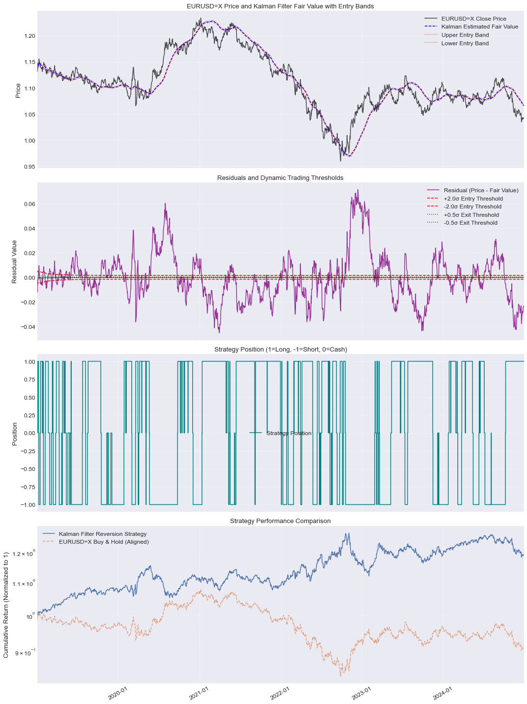
After generating signals, the script calculates daily strategy returns by multiplying the signal (position: +1 for long, -1 for short, 0 for cash) by the asset’s daily percentage change. These are then compounded to get cumulative returns. Performance metrics like annualized return, volatility, and Sharpe ratio are calculated for both the strategy and a simple buy-and-hold approach.

Finally, a series of plots help visualize:

1. The actual price against the Kalman Filter’s estimated fair value and the dynamic entry bands.

2. The residuals along with the entry and exit thresholds.

3. The strategy’s position over time (long, short, or cash).

4. The cumulative returns of the strategy compared to buy-and-hold.

These visualizations are crucial for understanding how the strategy behaves and whether it offers an advantage over simply holding the asset.

Conclusion

The Kalman Filter provides a sophisticated framework for estimating an asset’s underlying fair value in the face of noisy market data. By modeling this fair value and its trend, a mean reversion strategy can be built to capitalize on perceived mispricings. The provided Python script demonstrates a complete workflow, from data acquisition and filter application to signal generation and performance evaluation.

However, it’s important to remember that the success of such a strategy heavily depends on the correct parameterization of the Kalman Filter (especially the Q and R noise covariances) and the trading thresholds. These often require careful tuning and backtesting across various market conditions and assets. This approach is a powerful tool in the quantitative trader's arsenal but, like all models, it's an approximation of reality and should be used with a thorough understanding of its assumptions and limitations.