Apple's New Smart Display Confirms What This Startup Knew All Along

Apple has entered the smart home race with its new Smart Display, firing a $158B signal that connected homes are the future.

When Apple moves in, it doesn’t just join the market — it transforms it.

One company has been quietly preparing for this moment.

Their smart shade technology already works across every major platform, perfectly positioned to capture the wave of new consumers Apple will bring.

While others scramble to catch up, this startup is already shifting production from China to its new facility in the Philippines — built for speed and ready to meet surging demand as Apple’s marketing machine drives mass adoption.

With 200% year-over-year growth and distribution in over 120 Best Buy locations, this company isn’t just ready for Apple’s push — they’re set to thrive from it.

Shares in this tech company are open at just $1.90.

Apple’s move is accelerating the entire sector. Don’t miss this window.

Act Fast- Apple’s Halo effect is coming

_{Past performance is not indicative of future results. Email may contain forward-looking statements. See US Offering for details. Informational purposes only.}

🚀 Your Investing Journey Just Got Better: Premium Subscriptions Are Here! 🚀

It’s been 4 months since we launched our premium subscription plans at GuruFinance Insights, and the results have been phenomenal! Now, we’re making it even better for you to take your investing game to the next level. Whether you’re just starting out or you’re a seasoned trader, our updated plans are designed to give you the tools, insights, and support you need to succeed.

Here’s what you’ll get as a premium member:

• Exclusive Trading Strategies: Unlock proven methods to maximize your returns.

• In-Depth Research Analysis: Stay ahead with insights from the latest market trends.

• Ad-Free Experience: Focus on what matters most—your investments.

• Monthly AMA Sessions: Get your questions answered by top industry experts.

• Coding Tutorials: Learn how to automate your trading strategies like a pro.

• Masterclasses & One-on-One Consultations: Elevate your skills with personalized guidance.

Our three tailored plans—Starter Investor, Pro Trader, and Elite Investor—are designed to fit your unique needs and goals. Whether you’re looking for foundational tools or advanced strategies, we’ve got you covered.

Don’t wait any longer to transform your investment strategy. The last 4 months have shown just how powerful these tools can be—now it’s your turn to experience the difference.

👉 Explore Premium Plans Now

Introduction

In quantitative finance, risk management and volatility forecasting play a crucial role in designing trading strategies. This article explores a systematic approach to take-profit decisions using the Conditional Value at Risk (CVaR) on the right tail, also known as the Expected Upside Potential (EUP), combined with a Heterogeneous Auto-Regressive (HAR) model for volatility prediction.

We will analyze an equally weighted portfolio of the “Magnificent Seven” stocks and implement a data-driven methodology to determine dynamic sell signals.

Cut Through Noise with The Flyover!

• One Email with ALL the News

• Ditch the Mainstream Bias

• Quick, informative news that cuts through noise.

Subscribe with One Click!

1️. Data and Portfolio Construction

We start by selecting seven major tech stocks: Apple (AAPL), Microsoft (MSFT), NVIDIA (NVDA), Amazon (AMZN), Tesla (TSLA), Meta (META), and Alphabet (GOOGL). Using Yahoo Finance, we fetch historical adjusted closing prices from January 1, 2020, to March 15, 2025 and compute their daily returns.

import numpy as np
import pandas as pd
import yfinance as yf
import statsmodels.api as sm
import matplotlib.pyplot as plt

plt.close('all')

tickers = ["AAPL", "MSFT", "NVDA", "AMZN", "TSLA", "META", "GOOGL"]
data = yf.download(tickers, start="2020-01-01", end="2025-03-15", auto_adjust=False)["Close"]
returns = data.pct_change().dropna()

# Equally weighted portfolio
weights = np.ones(len(tickers)) / len(tickers)
portfolio_returns = returns.dot(weights)
portfolio_prices = (1 + portfolio_returns).cumprod() * 100  # Base 100

2️. Calculating VaR (95%) and Expected Upside Potential (EUP)

To quantify the risk and potential upside, we use:

• VaR (95%): The 95th percentile of rolling 60-day returns.

• EUP (Right-Tail CVaR): The average return of observations exceeding the 95th percentile.

window_eup = 60
rolling_var = portfolio_returns.rolling(window=window_eup).quantile(0.95)

def eup_cvar(x, alpha=95):
    threshold = np.percentile(x, alpha)
    tail = x[x >= threshold]
    return tail.mean() if len(tail) > 0 else np.nan

eup_series = portfolio_returns.rolling(window=window_eup).apply(lambda x: eup_cvar(x, alpha=95), raw=True)
signal = portfolio_returns > rolling_var  # Take-profit trigger

3️. HAR Model for Volatility Prediction

The Heterogeneous Auto-Regressive (HAR) Model is useful for forecasting daily volatility based on:

• Daily volatility (2-day window)

• Weekly volatility (5-day window)

• Monthly volatility (22-day window)

vol_daily   = portfolio_returns.rolling(window=2).std()
vol_weekly  = portfolio_returns.rolling(window=5).std()
vol_monthly = portfolio_returns.rolling(window=22).std()

vol_data = pd.DataFrame({
    'vol_daily': vol_daily,
    'vol_weekly': vol_weekly,
    'vol_monthly': vol_monthly
}).dropna()

X = sm.add_constant(vol_data[['vol_daily', 'vol_weekly', 'vol_monthly']])
y = vol_data['vol_daily'].shift(-1)
data_valid = pd.concat([X, y], axis=1).dropna()
X_valid = data_valid.iloc[:, :-1]
y_valid = data_valid.iloc[:, -1]

if len(X_valid) > 0:
    model = sm.OLS(y_valid, X_valid).fit()
    vol_data.loc[X_valid.index, 'vol_forecast'] = model.predict(X_valid)
else:
    vol_data['vol_forecast'] = np.nan

4️. Calculating the Sell Ratio and Sale Percentage

We compute the sell ratio as:

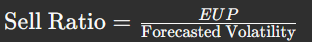
The ratio is mapped to a sale percentage between 0% and 100%, based on predefined thresholds:

• Sell Ratio ≤ 1.0 → 0% Sale

• Sell Ratio ≥ 3.0 → 100% Sale

• Between 1.0 and 3.0 → Interpolated proportionally

common_index = portfolio_returns.index.intersection(vol_data['vol_forecast'].dropna().index)
eup_aligned = eup_series.loc[common_index]
signal_aligned = signal.loc[common_index]
vol_forecast_aligned = vol_data['vol_forecast'].loc[common_index]

ratio = pd.Series(np.nan, index=common_index)
for date in common_index:
    if signal_aligned.loc[date]:
        if not pd.isna(eup_aligned.loc[date]) and not pd.isna(vol_forecast_aligned.loc[date]):
            ratio.loc[date] = eup_aligned.loc[date] / vol_forecast_aligned.loc[date]

def sale_percentage(r, threshold_min=1.0, threshold_max=3.0):
    if r <= threshold_min:
        return 0.0
    elif r >= threshold_max:
        return 1.0
    else:
        return (r - threshold_min) / (threshold_max - threshold_min)

sales_percentage = ratio.dropna().apply(sale_percentage)

5️. Printing and Visualizing Sell Signals

print("Last 10 Sell Ratios (EUP / Volatility Forecast):")
print(ratio.dropna().tail(10))
print("\nLast 10 Sale Percentages:")
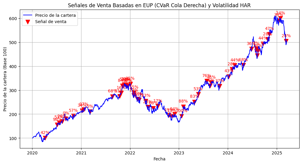
print(sales_percentage.tail(10))

We plot the portfolio price evolution, highlighting sell signals with red markers:

fig, ax = plt.subplots(figsize=(12, 6))
ax.plot(portfolio_prices.index, portfolio_prices, label="Portfolio Price", color="blue")

sales_dates = sales_percentage.index
if not sales_dates.empty:
    ax.scatter(sales_dates, portfolio_prices.loc[sales_dates],
               color="red", marker="v", s=100, label="Sell Signal")
    for date in sales_dates:
        perc = sales_percentage.loc[date] * 100
        ax.annotate(f"{perc:.0f}%", (date, portfolio_prices.loc[date]),
                    textcoords="offset points", xytext=(0,10), ha="center", color="red")

ax.set_title("Sell Signals Based on EUP (Right-Tail CVaR) and HAR Volatility Model")
ax.set_xlabel("Date")
ax.set_ylabel("Portfolio Price (Base 100)")
ax.legend()
ax.grid(True)
plt.show()

Conclusion

This approach integrates EUP-based take-profit signals with a HAR volatility model to adaptively determine optimal sell percentages. Unlike fixed thresholds, this data-driven strategy adjusts dynamically to market conditions, offering a more systematic way to take profits based on expected upside potential and forecasted risk.