Kickstart your holiday campaigns

CTV should be central to any growth marketer’s Q4 strategy. And with Roku Ads Manager, launching high-performing holiday campaigns is simple and effective.

With our intuitive interface, you can set up A/B tests to dial in the most effective messages and offers, then drive direct on-screen purchases via the remote with shoppable Action Ads that integrate with your Shopify store for a seamless checkout experience.

Don’t wait to get started. Streaming on Roku picks up sharply in early October. By launching your campaign now, you can capture early shopping demand and be top of mind as the seasonal spirit kicks in.

Get a $500 ad credit when you spend your first $500 today with code: ROKUADS500. Terms apply.

Holiday performance starts now.

🚀 Your Investing Journey Just Got Better: Premium Subscriptions Are Here! 🚀

It’s been 4 months since we launched our premium subscription plans at GuruFinance Insights, and the results have been phenomenal! Now, we’re making it even better for you to take your investing game to the next level. Whether you’re just starting out or you’re a seasoned trader, our updated plans are designed to give you the tools, insights, and support you need to succeed.

Here’s what you’ll get as a premium member:

• Exclusive Trading Strategies: Unlock proven methods to maximize your returns.

• In-Depth Research Analysis: Stay ahead with insights from the latest market trends.

• Ad-Free Experience: Focus on what matters most—your investments.

• Monthly AMA Sessions: Get your questions answered by top industry experts.

• Coding Tutorials: Learn how to automate your trading strategies like a pro.

• Masterclasses & One-on-One Consultations: Elevate your skills with personalized guidance.

Our three tailored plans—Starter Investor, Pro Trader, and Elite Investor—are designed to fit your unique needs and goals. Whether you’re looking for foundational tools or advanced strategies, we’ve got you covered.

Don’t wait any longer to transform your investment strategy. The last 4 months have shown just how powerful these tools can be—now it’s your turn to experience the difference.

👉 Explore Premium Plans Now

In a previous article, we explored the ARCH model and how it can be used to model and predict volatility in financial time series data. While ARCH was groundbreaking (Robert Engle won the Nobel prize for it), it also had several limitations:

• Financial time series often exhibit long memory in volatility. ARCH cannot effectively capture it without including many lags.

• ARCH ignores the leverage effect, assuming that positive and negative shocks of the same magnitude have identical impacts on volatility.

• ARCH does not effectively explain variations in volatility, making it prone to over-forecasting. This is because it responds slowly to large, isolated shocks in the returns series.

In this article, we’ll explore a new class of models designed to address the first of these issues.

Wall Street has Bloomberg. You have Stocks & Income.

Why spend $25K on a Bloomberg Terminal when 5 minutes reading Stocks & Income gives you institutional-quality insights?

We deliver breaking market news, key data, AI-driven stock picks, and actionable trends—for free.

Subscribe for free and take the first step towards growing your passive income streams and your net worth today.

Get Free Daily Market Updates →

_{Stocks & Income is for informational purposes only and is not intended to be used as investment advice. Do your own research.}

📚 The GARCH Model

In 1986, Tim Bollerslev introduced the GARCH model, which stands for Generalized Autoregressive Conditional Heteroskedasticity. While ARCH models the conditional variance as a function of past squared residuals, GARCH also incorporates lagged conditional variances. As such, GARCH consists of two components:

• The ARCH part (past squared residuals) corresponding to short-term shocks,

• The GARCH part (lagged conditional variances) accounting for the long-term persistence.

The formula of the standard GARCH(p, q) looks as follows:

Where:

• σ_t² ​ is the conditional variance at time t,

• ε_t is the error term (residual) at time t,

• α_0 > 0, α_i ≥ 0, and β_i ≥ 0 are parameters to be estimated.

To get a better understanding of the formula, let’s look at the simplest GARCH model, that is, GARCH(1,1).

The formula essentially states that today’s volatility depends on three elements:

• A constant (α_0) that represents the long-term average volatility,

• The squared shock from yesterday,

• Yesterday’s conditional variance.

Something that we should be aware of is an assumption regarding the parameters of the model. For the GARCH process to be weakly stationary, the sum of the ARCH and GARCH coefficients must be less than 1. Satisfying this condition makes sure that the conditional variance reverts to a finite long-run average.

The closer the sum of the parameters gets to 1, the higher the persistence. Volatility persistence refers to how long the effect of a shock lasts in future volatility estimates. Let’s look at two examples:

• A persistent process means that once volatility increases, it remains elevated for a long time.

• A low persistence process means volatility quickly reverts to its average level.

Before wrapping up the theoretical part, let’s briefly look at the advantages and disadvantages of GARCH models.

Pros:

• GARCH models effectively capture volatility clustering.

• They are more flexible than ARCH models and require fewer parameters to be estimated (i.e., fewer lags).

• They result in better long-term forecasts compared to pure ARCH.

Cons:

• GARCH assumes symmetry — positive and negative shocks are treated equally.

• Similar to ARCH, it does not account for leverage effects (reminder: the tendency for volatility to increase more following bad news than good news).

• GARCH models tend to miss extreme events. As such, the models underestimate kurtosis and therefore may not fully capture fat tails.

• Parameter estimation can be computationally intensive.

💻 Hands-On Example in Python

Just as we did last time when estimating ARCH models, we will be using the arch library.

As always, we start by importing the required libraries: requests to download data, pandas for some data wrangling, matplotlib for plotting, and, arch for volatility forecasting.

The api_key file contains our personal API key to Financial Modelling Prep’s API, from where we will download the historical stock prices.

import requests
import pandas as pd
from arch import arch_model
from datetime import datetime

# plotting
import matplotlib.pyplot as plt

# settings
plt.style.use("seaborn-v0_8-colorblind")
plt.rcParams["figure.figsize"] = (16, 8)

# api key
from api_keys import FMP_API_KEY

Then, we download the data. For this example, we use Apple’s stock prices from 2015 to April 2025. ARCH/GARCH models estimate time-varying variance, which is generally more data-hungry than conditional mean models. With too little data, we risk unstable variance estimates and overfitting. Having enough data also helps capture different volatility regimes.

TICKER = "AAPL"
START_DATE = "2015-01-01"
END_DATE = "2025-04-30"
SPLIT_DATE = datetime(2025, 1, 1)

def get_adj_close_price(symbol: str, start_date: str, end_date: str) -> pd.DataFrame:
    """
    Fetches adjusted close prices for a given ticker and date range from FMP.
    """
    url = f"https://financialmodelingprep.com/api/v3/historical-price-full/{symbol}"
    params = {
        "from": start_date,
        "to": end_date,
        "apikey": FMP_API_KEY
    }
    response = requests.get(url, params=params)
    r_json = response.json()

    if "historical" not in r_json:
        raise ValueError(f"No historical data found for {symbol}")

    df = pd.DataFrame(r_json["historical"]).set_index("date").sort_index()
    df.index = pd.to_datetime(df.index)
    return df[["adjClose"]].rename(columns={"adjClose": symbol})


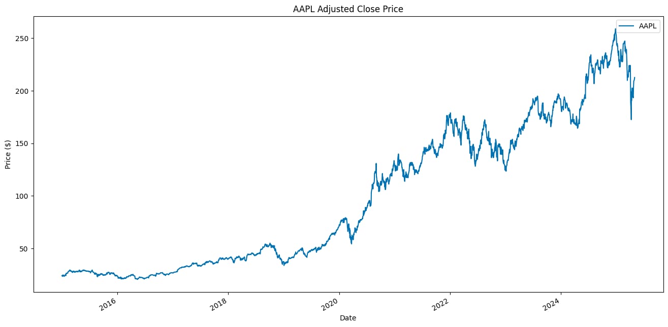
price_df = get_adj_close_price(TICKER, START_DATE, END_DATE)
price_df.plot(title=f"{TICKER} Adjusted Close Price", ylabel="Price ($)", xlabel="Date")

Below we can see the downloaded stock prices of Apple.

Then, we need to convert the prices to returns.

return_df = 100 * price_df[TICKER].pct_change().dropna()
return_df.name = "asset_returns"
return_df.plot(title=f"{TICKER} returns - {START_DATE}:{END_DATE}");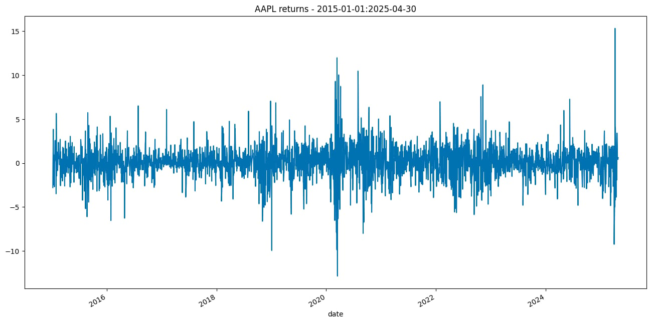

In this exercise, we compare the ARCH(1) model with the GARCH(1,1) model. Thanks to the flexibility of the arch library, we can easily estimate multiple models with minimal changes to the function call.

model_1 = arch_model(return_df, mean="Constant", vol="ARCH", p=1, q=0)
model_2 = arch_model(return_df, mean="Constant", vol="GARCH", p=1, q=1)

fitted_model_1 = model_1.fit(disp="off")
fitted_model_2 = model_2.fit(disp="off")

While calling the arch_model function, we specified the following:

• p — Number of lagged squared residuals (ARCH terms).

• q — Number of lagged conditional variances (GARCH terms).

• mean — This argument controls the mean equation of the time series, that is, how the returns are modeled. In this case, we decided to use a constant mean model. This means that we are assuming that the return series has a constant (non-zero) mean, and we are not modeling any dynamics in the mean process, for example, with AR or MA behavior. Another option could be to use the zero-mean model.

• vol —With this argument, we specified which type of volatility model we are using.

We can inspect the fitted models by using the summary method.

print(fitted_model_1.summary())

For the ARCH model, we see the following summary:

                      Constant Mean - ARCH Model Results                      
==============================================================================
Dep. Variable:          asset_returns   R-squared:                       0.000
Mean Model:             Constant Mean   Adj. R-squared:                  0.000
Vol Model:                       ARCH   Log-Likelihood:               -5148.40
Distribution:                  Normal   AIC:                           10302.8
Method:            Maximum Likelihood   BIC:                           10320.4
                                        No. Observations:                 2596
Date:                Sun, Jul 13 2025   Df Residuals:                     2595
Time:                        12:58:03   Df Model:                            1
                                Mean Model                                
==========================================================================
                 coef    std err          t      P>|t|    95.0% Conf. Int.
--------------------------------------------------------------------------
mu             0.1445  3.596e-02      4.018  5.857e-05 [7.403e-02,  0.215]
                            Volatility Model                            
========================================================================
                 coef    std err          t      P>|t|  95.0% Conf. Int.
------------------------------------------------------------------------
omega          2.4765      0.167     14.820  1.092e-49 [  2.149,  2.804]
alpha[1]       0.2702  5.895e-02      4.583  4.590e-06 [  0.155,  0.386]
========================================================================

Covariance estimator: robust

And then we generate a similar summary for the GARCH model:

                     Constant Mean - GARCH Model Results                      
==============================================================================
Dep. Variable:          asset_returns   R-squared:                       0.000
Mean Model:             Constant Mean   Adj. R-squared:                  0.000
Vol Model:                      GARCH   Log-Likelihood:               -4994.00
Distribution:                  Normal   AIC:                           9996.00
Method:            Maximum Likelihood   BIC:                           10019.4
                                        No. Observations:                 2596
Date:                Sun, Jul 13 2025   Df Residuals:                     2595
Time:                        12:58:03   Df Model:                            1
                                Mean Model                                
==========================================================================
                 coef    std err          t      P>|t|    95.0% Conf. Int.
--------------------------------------------------------------------------
mu             0.1616  3.255e-02      4.966  6.847e-07 [9.784e-02,  0.225]
                             Volatility Model                             
==========================================================================
                 coef    std err          t      P>|t|    95.0% Conf. Int.
--------------------------------------------------------------------------
omega          0.1595  5.555e-02      2.871  4.089e-03 [5.062e-02,  0.268]
alpha[1]       0.1121  2.540e-02      4.415  1.010e-05 [6.236e-02,  0.162]
beta[1]        0.8400  3.636e-02     23.100 4.588e-118   [  0.769,  0.911]
==========================================================================

Covariance estimator: robust

In the next step, we can inspect the standardized residuals and the conditional volatility series by plotting them. The standardized residuals are computed by dividing the residuals by the conditional standard deviation.

We use the annualize="D" argument of the plot method to annualize the conditional volatility series from daily data.

fitted_model_1.plot(annualize="D");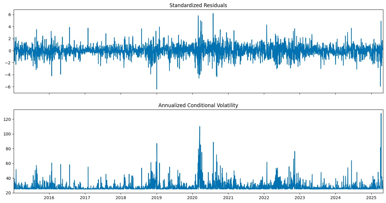

You might wonder how to interpret such a plot. In an ideal scenario, the standardized residuals should resemble white noise, that is, they should have a mean of zero and exhibit constant variance over time. The absence of any clear patterns or trends suggests that the model has adequately captured the volatility structure of the returns.

Let’s look at the plots of the GARCH model now.

fitted_model_2.plot(annualize="D");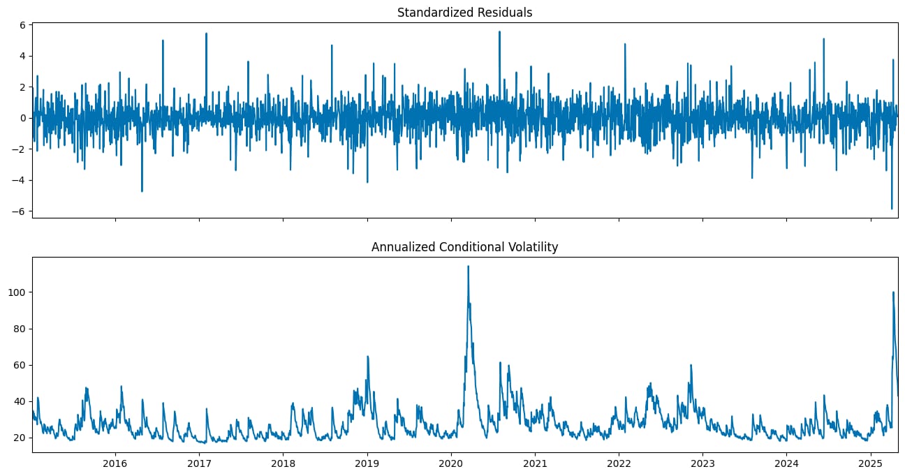

Having estimated the models, it is now time to generate the volatility forecasts. Using the ARCH/GARCH models, there are three main approaches to doing so:

• Analytical: One-step forecasts are always available due to the model structure. Multi-step forecasts require forward recursion and are only feasible for models that are linear in squared residuals. While this method is not suitable for pure ARCH models, it can be used with GARCH models (and some of their extensions).

• Simulation: This approach simulates future volatility paths using random draws from a specified residual distribution. Averaging these paths yields the forecast. It works for any forecast horizon and converges to the analytical forecast as the number of simulations increases.

• Bootstrap (aka, Filtered Historical Simulation): Similar to simulation, but draws standardized residuals from historical data using the estimated model parameters. This method requires only a small amount of in-sample data.

Due to the specification of ARCH/GARCH models, the first out-of-sample forecast will always be the same, regardless of which approach we use.

As you can see in the snippet below, we use the “analytic” method for generating the forecasts, but you could also pass in “simulation” or “bootstrap”.

Another important point is that we are refitting the models. This is done to train the model on a subset of the data and then use it to make predictions on the remaining portion, effectively creating a train-test split. Specifically, we will train the models using 10 years of data up to the end of 2024, and then begin making predictions starting on January 1st, 2025.

fitted_model_1 = model_1.fit(last_obs=SPLIT_DATE, disp="off")
fitted_model_2 = model_2.fit(last_obs=SPLIT_DATE, disp="off")

forecasts_analytical_1 = fitted_model_1.forecast(
    horizon=1,
    start=SPLIT_DATE,
    method="analytic",
    reindex=False
)

forecasts_analytical_2 = fitted_model_2.forecast(
    horizon=1,
    start=SPLIT_DATE,
    method="analytic",
    reindex=False
)

a = forecasts_analytical_1.variance.rename(columns={"h.1": "arch(1)"})
b = forecasts_analytical_2.variance.rename(columns={"h.1": "garch(1,1)"})
a.join(b).plot(title="Analytical forecasts for horizon = 1");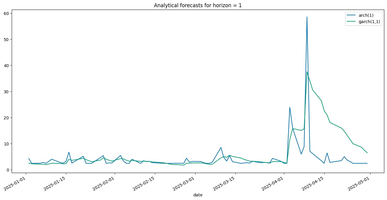

As you can see in the generated plot, the volatility forecast varies quite a lot depending on the choice of the model.

📈 A note about using GARCH to predict returns

At this point, you might be asking: Can a GARCH model be used on its own to predict returns? The answer is: yes and no.

In the approach we used above, we assumed that returns have a constant mean. However, in reality, this assumption doesn’t always hold, and it fails to fully capture characteristics like skewness and leptokurtosis (fat tails and a sharp peak in the return distribution) present in financial time series.

This is why ARMA and GARCH models are often combined. The ARMA model estimates the conditional mean, while the GARCH model captures the conditional variance in the residuals of the ARMA model.

A practical — but often overlooked — point concerns how to estimate this combination. One approach is to first fit an ARMA model and then apply a GARCH model to its residuals. However, this is not recommended, as the ARMA estimates will generally be inconsistent, which in turn contaminates the GARCH estimates.

The preferred approach is to estimate the ARMA and GARCH models jointly, ensuring consistent and efficient parameter estimates.

There is one exception: when the mean model includes only AR terms (and no MA terms). In that case, the estimates will still be consistent, but not efficient.

Wrapping up

In this article, we have explored volatility forecasting with GARCH models. The main takeaways are:

• The GARCH model extends ARCH by modeling current volatility as a function of both past squared errors and past variances.

• It provides a more parsimonious and stable way to forecast volatility compared to high-order ARCH models. By doing so, it often requires fewer parameters to be estimated.

• GARCH effectively models persistent volatility and clustering, making it widely used in financial applications such as risk forecasting, Value at Risk, and derivative pricing.

You can find the code used in this article in this repository.