Modernize your marketing with AdQuick

AdQuick unlocks the benefits of Out Of Home (OOH) advertising in a way no one else has. Approaching the problem with eyes to performance, created for marketers with the engineering excellence you’ve come to expect for the internet.

Marketers agree OOH is one of the best ways for building brand awareness, reaching new customers, and reinforcing your brand message. It’s just been difficult to scale. But with AdQuick, you can easily plan, deploy and measure campaigns just as easily as digital ads, making them a no-brainer to add to your team’s toolbox.

Learn more now.

🚀 Your Investing Journey Just Got Better: Premium Subscriptions Are Here! 🚀

It’s been 4 months since we launched our premium subscription plans at GuruFinance Insights, and the results have been phenomenal! Now, we’re making it even better for you to take your investing game to the next level. Whether you’re just starting out or you’re a seasoned trader, our updated plans are designed to give you the tools, insights, and support you need to succeed.

Here’s what you’ll get as a premium member:

• Exclusive Trading Strategies: Unlock proven methods to maximize your returns.

• In-Depth Research Analysis: Stay ahead with insights from the latest market trends.

• Ad-Free Experience: Focus on what matters most—your investments.

• Monthly AMA Sessions: Get your questions answered by top industry experts.

• Coding Tutorials: Learn how to automate your trading strategies like a pro.

• Masterclasses & One-on-One Consultations: Elevate your skills with personalized guidance.

Our three tailored plans—Starter Investor, Pro Trader, and Elite Investor—are designed to fit your unique needs and goals. Whether you’re looking for foundational tools or advanced strategies, we’ve got you covered.

Don’t wait any longer to transform your investment strategy. The last 4 months have shown just how powerful these tools can be—now it’s your turn to experience the difference.

👉 Explore Premium Plans Now

In my previous article, I tested a simple 2-day SMA crossover strategy on Tesla stock. Even after factoring in slippage and commissions, the strategy still managed to stay profitable — surprisingly so.

But was that a fluke unique to TSLA’s chaotic price action?

This time, I applied the same setup to a few other major tech stock to find out.

Missed the Market’s Big Moves?

The market moves fast - we make sure you don’t miss a thing.

Elite Trade Club delivers clear, no-fluff market intel straight to your inbox every morning.

From stocks to big-picture trends, we cover what actually matters.

Join 100,000+ readers who start their day with the edge.

Click Here to Join Now

So here’s the code used for this analysis

import yfinance as yf
import numpy as np
import pandas as pd
import matplotlib.pyplot as plt

def sma_strategy_slippage_commission(df_org,window,slippage_rate,commission_rate,draw = True):
    df = df_org.copy()
    # Calculate SMA based on closing price
    df['SMA'] = df.rolling(window=window).mean().fillna(0)

    # Calculate execution price with slippage (assume buying slightly worse than close)
    df['ExecPrice'] = df[ticker] * (1 - slippage_rate)
    
    # Generate signal using ideal (close) price
    df['Signal'] = (df[ticker] < df['SMA']).astype(int)
    df['Position'] = df['Signal'].diff()

    # Buy and sell points using slippage-adjusted execution price
    df['Buy'] = (df['Position'] == 1).astype(int)*df['ExecPrice']
    df['Sell'] = (df['Position'] == -1).astype(int)*df['ExecPrice']
    
    # If there is a final unmatched Buy, we force-close it at the last available price
    if (df['Buy'] - df['Sell'] ).sum() > 0:
        df['Sell'].iat[-1] = df['ExecPrice'].iat[-1]

    # Compute commissions for each trade
    df['Buy_commission'] = df['Buy'] * commission_rate
    df['Sell_commission'] = df['Sell'] * commission_rate

    # Calculate profit net of slippage and commissions
    df['Profit'] = (df['Sell'] - df['Buy'] - df['Buy_commission'] - df['Sell_commission']).cumsum()
    df['Profit on sale'] = ((df['Sell'] > 0).astype(int)*df['Profit']).cumsum()

    if draw is True:
        fig,axs = plt.subplots(2,1,figsize=(14,8))
        ax = axs[0]
        ax.plot(df.index,df[ticker],label = ticker ,color='black')
        ax.plot(df.index[window:],df['SMA'][window:],label = 'SMA' ,color='grey')
        ax.scatter(df.index,(df['Buy']).replace(0,np.nan),label='Buy',color='blue')
        ax.scatter(df.index,(df['Sell']).replace(0,np.nan),label='Sell',color='red')
        ax.label_outer()
        ax.set_title('SMA Crossover Strategy: '+str(ticker))
        ax.set_ylabel('Price')
        ax.grid()
        ax.legend()
        
        ax = axs[1]
        ax.plot(df.index,df['Profit on sale'])
        ax.set_ylabel('Pofit')
        ax.set_xlabel('Date')
        ax.grid()
    
    return df

Quick Comparison Across Stocks

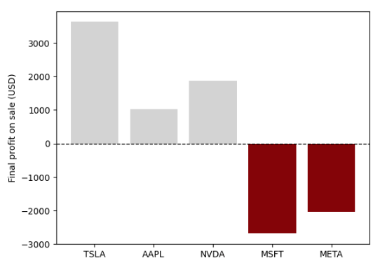
I ran the strategy across five major tickers: TSLA, AAPL, MSFT, and META.

Here’s a simple bar chart comparing their final profits (after accounting for slippage and commissions):

tickers = ['TSLA','AAPL','NVDA','MSFT','META']
window = 2
slippage_rate = 0.001
commission_rate = 0.001

fig, ax = plt.subplots()
ax.axhline(0, color='black', linestyle='--', linewidth=1)
ax.set_ylabel('Final profit on sale (USD)')
color = 'lightgrey'
prof_df = pd.DataFrame(index=tickers)
ys = []
for ticker in tickers:
    df_org = yf.download(ticker, start="2024-04-01", end="2025-06-07")['Close']
    df = sma_strategy_slippage_commission(df_org,window,slippage_rate,commission_rate,False)
    y = df['Profit on sale'].iat[-1]
    ys.append(y)
    color = 'lightgrey' if 0 <= y else 'darkred'
    ax.bar(ticker,y,color=color)
prof_df['Final profit on sale'] = ys

The differences were bigger than I expected. Here’s how each stock performed under the same 2-day SMA strategy:

Why Did These Two Lose Money?

While TSLA, AAPL, and NVDA stayed in the green, MSFT and META ended up losing money under the same conditions.

Here’ a quick dive into why.

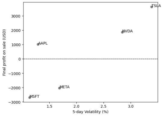
To investigate further, I plotted each stock’s final profit against its 5-day volatility.

The idea: maybe the more chaotic stocks just happened to benefit from the strategy.

tickers = ['TSLA','AAPL','NVDA','MSFT','META']
start_date = "2024-04-01"
end_date = "2025-06-07"

volatility = {}

for ticker in tickers:
    df = yf.download(ticker, start=start_date, end=end_date)['Close']
    returns = df.pct_change().dropna()
    vol = returns.rolling(window=2).std().mean()
    volatility[ticker] = vol[ticker]

vol_df = pd.DataFrame.from_dict(volatility, orient='index', columns=['5-day Volatility'])

fig, ax = plt.subplots()
ax.axhline(0, color='black', linestyle='--', linewidth=1)
ax.set_xlabel('5-day Volatility (%)')
ax.set_ylabel('Final profit on sale (USD)')
for ticker in prof_df.index:
    x = vol_df['5-day Volatility'][ticker]*100
    y = prof_df['Final profit on sale'][ticker]
    ax.scatter(x,y,color='grey')
    ax.text(x,y,ticker)

Here’s what that looks like visually: each dot represents one tech stock, showing how volatility might relate to strategy performance.

What This Tells Us

Despite the simplicity of the 2-day SMA, it manages to capture meaningful signals — especially when paired with volatile stocks.

It doesn’t work across the board, as seen with MSFT and META, but when the market’s noisy, reacting quickly seems to pay off.

In that sense, this isn’t just a strategy — it’s a vibe check.

If the market’s calm, a reactive system like this one might just fizzle out.

But in chaos? It thrives.

Maybe that’s deeper lesson:

Volatility isn’t a bug — it’s the feature this strategy is built to exploit.